The first eleven chapters each covered one part of making a chart. This chapter applies those parts in order to a single dataset, from the first exploratory chart to the final caption. It also shows the intermediate drafts, including the ones that are discarded. The dataset is life expectancy at birth for every country since 1950. Our World in Data compiled it from the UN World Population Prospects and the Human Mortality Database (Roser, Ortiz-Ospina, and Ritchie, 2013, updated 2023). It has about 18,000 rows. The worked example concerns the United States and its position among countries of similar income.
The chapter also sets out a method for working with language models that draw charts. Each earlier chapter ended with a short warning about these tools. This chapter ends with a set of rules for using them.
12.2 Step 1: Look Before Asking
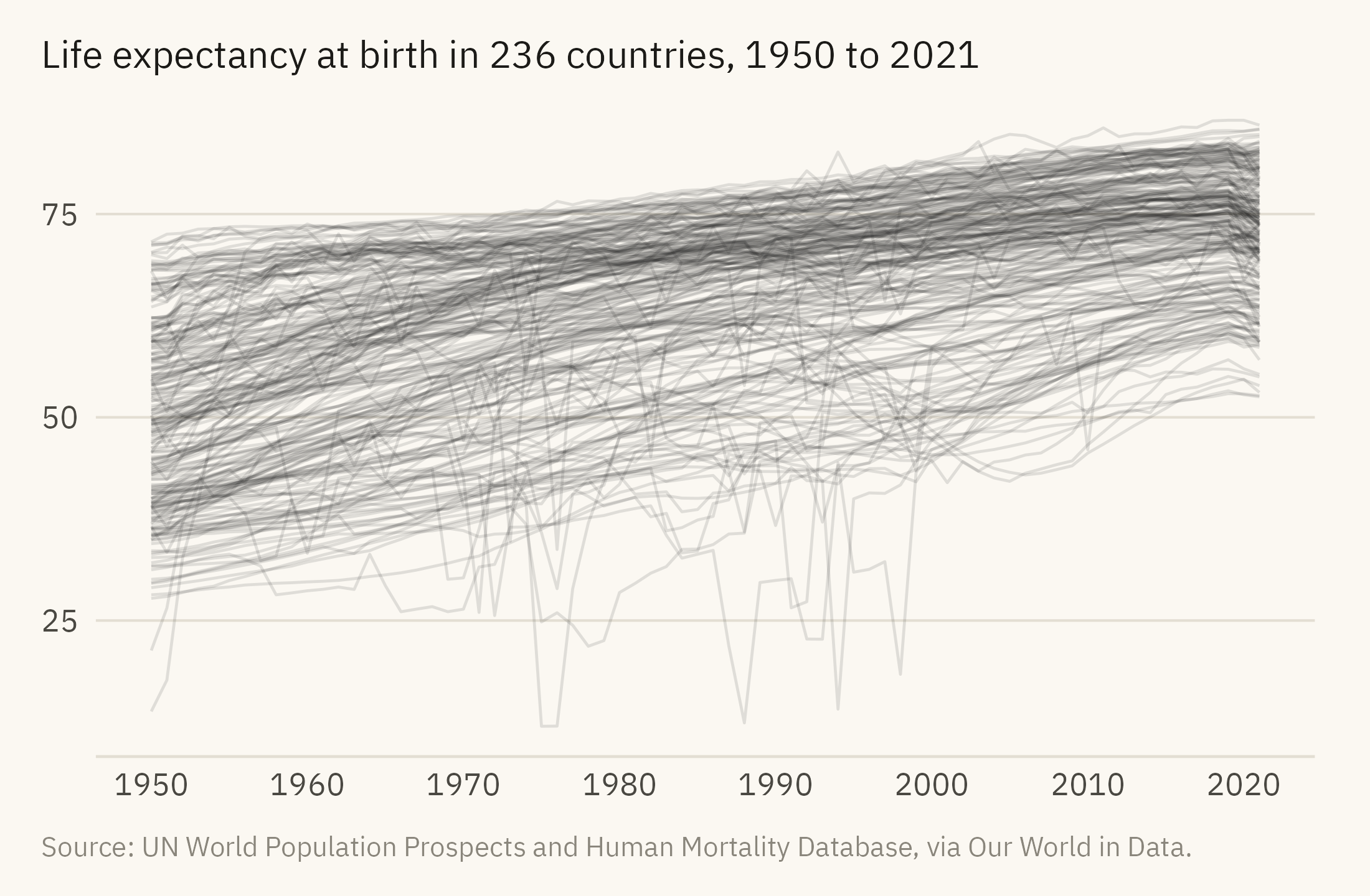
The first chart is drawn for the author rather than for a reader. Figure 12.1 draws every country as a line. Chapter 1 called a line chart with this many series a spaghetti chart, since no single line can be followed. It is not a chart to publish. It is a chart to look at for a minute before deciding what to ask. From it a reader can see the lowest and highest values in the data, roughly 12 and 87 years, and the broad movements over seventy years.
Show the code
ggplot(countries, aes(year, life_expectancy, group = country)) +geom_line(color = mv_ink$ink, alpha =0.12, linewidth =0.4) +scale_x_continuous(breaks =seq(1950, 2020, 10)) +labs(title =paste0("Life expectancy at birth in ", n_distinct(countries$country), " countries, 1950 to 2021"), x =NULL, y =NULL, caption =mv_source(src)) +theme_mv() + plain_title
Figure 12.1: Life expectancy at birth for every country, 1950 to 2021, one line each. This is an exploration chart. A reader can see that nearly every line rises, that the spread narrowed, and that many lines fall in 2020 and 2021. No single line can be identified. Source: UN World Population Prospects and Human Mortality Database, via Our World in Data.
Three things can be seen in Figure 12.1, and a story could be written about any of them. Most lines rise, which is the global gain in life expectancy since 1950. The lines are closer together in 2021 than in 1950, which is convergence between countries. Many lines drop in 2020 and 2021, which is the pandemic. A fourth possible story does not come from the chart. High-income countries are at the top of the chart, and the United States is a high-income country. This chapter asks whether the United States is where its income would place it.
12.3 Step 2: Choose the Comparison
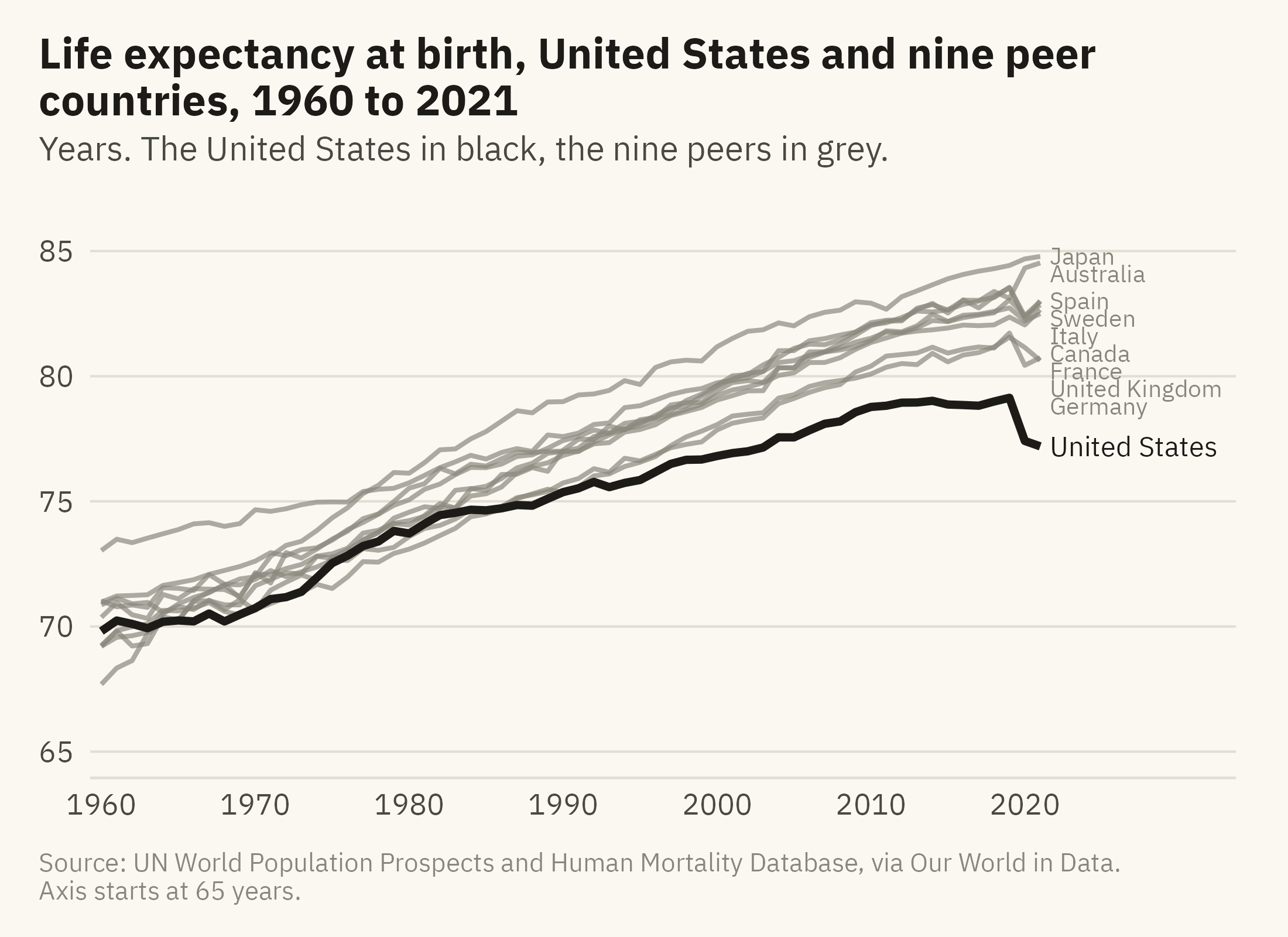
To say that one country is ahead or behind, you have to say compared with whom. Compared with the world average, the United States is well ahead, because most countries are poorer. Compared with the ten countries with the longest lives, almost every country is behind. Neither comparison answers the question. The fair comparison is with countries of similar income that also keep reliable death records. I use nine: Japan, Australia, Italy, Spain, Sweden, France, Canada, Germany, and the United Kingdom. Figure 12.2 shows them with the United States. The caption names them so a reader can object to the list.
Show the code
# Space the end labels by hand: sort by value and push each one down until# it clears the one above it by 0.7 years.ends <- rich |>filter(year ==2021) |>arrange(desc(life_expectancy)) |>mutate(label_y = life_expectancy)for (i inseq_len(nrow(ends))[-1]) { ends$label_y[i] <-min(ends$label_y[i], ends$label_y[i -1] -0.7)}ends <- ends |>mutate(is_us = country =="United States",col =if_else(is_us, mv_accent(), mv_ink$mute),sz =if_else(is_us, 3, 2.6))ggplot(rich, aes(year, life_expectancy, group = country)) +geom_line(data =filter(rich, country !="United States"), color = mv_ink$mute, linewidth =0.7, alpha =0.7) +geom_line(data =filter(rich, country =="United States"), color =mv_accent(), linewidth =1.2) +geom_text(data = ends, aes(x =2021.6, y = label_y, label = country), color = ends$col,size = ends$sz, hjust =0, family =mv_font()) +scale_x_continuous(breaks =seq(1960, 2020, 10), limits =c(1960, 2033), expand =expansion(mult =0.01)) +scale_y_continuous(limits =c(65, 86)) +labs(title ="Life expectancy at birth, United States and nine peer countries, 1960 to 2021",subtitle ="Years. The United States in black, the nine peers in grey.",x =NULL, y =NULL, caption =paste0(mv_source(src), "\nAxis starts at 65 years.")) +theme_mv()
Figure 12.2: Life expectancy at birth in the United States and nine peer countries, 1960 to 2021. The peers are Japan, Australia, Italy, Spain, Sweden, France, Canada, Germany, and the United Kingdom. In 1960 the United States was sixth of the ten. From the late 1980s it has been at the bottom. The gap has widened since. Source: UN World Population Prospects and Human Mortality Database, via Our World in Data.
The chart form follows Chapter 9. The United States is the one dark line, the nine peers are in grey, and direct labels replace a legend. This chapter’s accent is black, the ink of the finished story. The vertical axis starts at 65 years, and the caption says so. Chapter 7 gives the rule for this choice. A line chart may start its axis above zero when the reader can see the reason. Here every value lies between 67 and 85 years. An axis from zero would place all ten lines in a narrow band at the top of the panel. The differences between them would then be hard to read.
12.4 Step 3: Find the Shape of the Gap
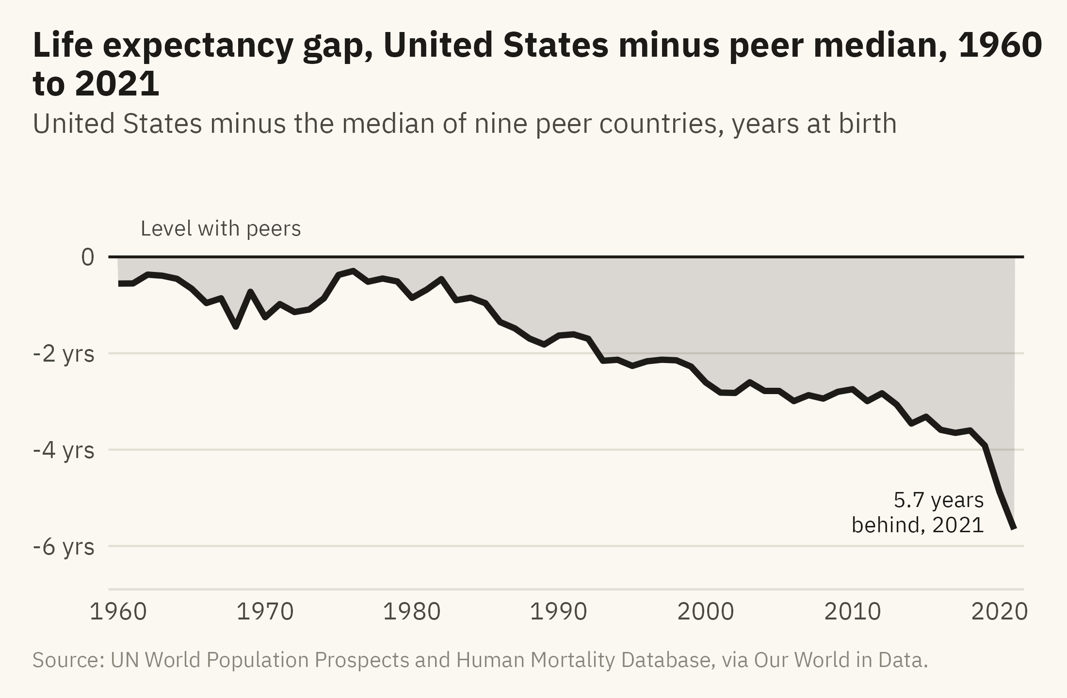
Figure 12.2 shows ten lines, and the question is how far the United States line is from the other nine. In that chart a reader has to judge the distance by eye, between lines that cross and bunch together. Chapter 7 recommends computing the difference and plotting it when the difference is the question. Figure 12.3 does that. For each year it subtracts the median of the nine peers from the United States value.
Show the code
gap <- rich |>group_by(year) |>summarise(us = life_expectancy[country =="United States"],peer =median(life_expectancy[country !="United States"]), .groups ="drop") |>mutate(gap = us - peer)ggplot(gap, aes(year, gap)) +geom_hline(yintercept =0, color = mv_ink$ink, linewidth =0.5) +geom_area(fill =mv_accent(), alpha =0.15) +geom_line(color =mv_accent(), linewidth =1.1) +annotate("text", x =1967, y =0.6, label ="Level with peers", size =2.9, family =mv_font(), color = mv_ink$ink2) +annotate("text", x =2019, y =-5.3, label =sprintf("%.1f years\nbehind, 2021", -last(gap$gap)), hjust =1, size =2.9,family =mv_font(), color =mv_accent(), lineheight =0.95) +scale_x_continuous(breaks =seq(1960, 2020, 10), expand =expansion(mult =0.01)) +scale_y_continuous(limits =c(-6.5, 1.5), breaks =c(-6, -4, -2, 0), labels = \(x) if_else(x ==0, "0", paste0(x, " yrs"))) +labs(title ="Life expectancy gap, United States minus peer median, 1960 to 2021",subtitle ="United States minus the median of nine peer countries, years at birth",x =NULL, y =NULL, caption =mv_source(src)) +theme_mv()
Figure 12.3: The United States minus the median of its nine peers, in years of life expectancy at birth, 1960 to 2021. The gap stayed within about a year of zero through the 1970s. It opened steadily from 1980 and reached three years in 2013. In 2021 it reached 5.7 years. Source: UN World Population Prospects and Human Mortality Database, via Our World in Data.
Figure 12.3 is the main chart of the story. A reader who sees only this chart can learn the finding, its size, and its timing. The gap stayed within about a year of zero through the 1970s, reached three years in 2013, and reached 5.7 years in 2021. Nothing in the chart says why the gap opened. The caption should not say either.
12.5 Step 4: Ask What the Chart Leaves Out
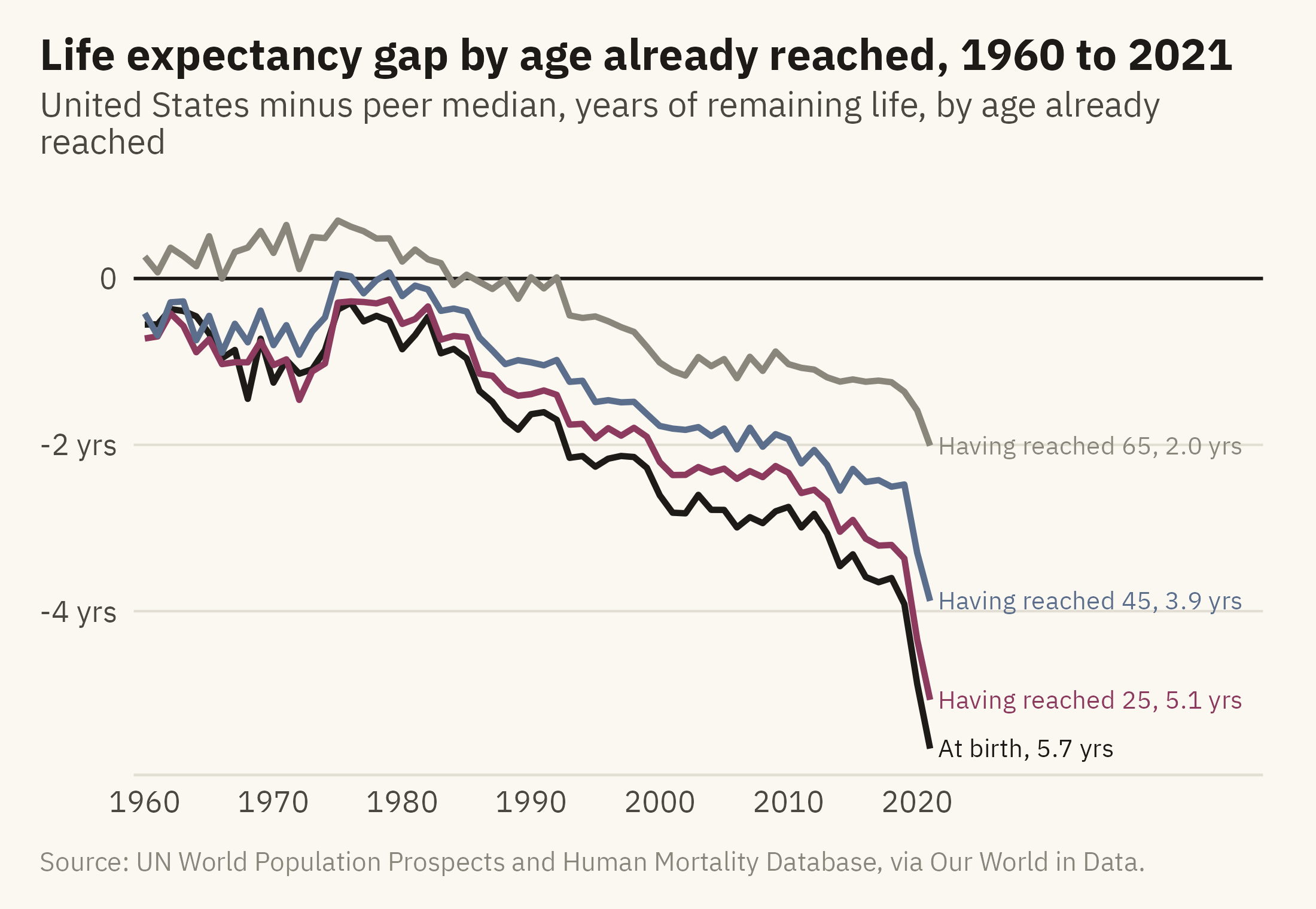
Before publishing, I apply the seven questions from Chapter 3 to my own chart. What is counted? Period life expectancy, which is the age a newborn would reach if the death rates of a single year held for that newborn’s whole life. It describes the deaths of one year. It is not a prediction for the babies born that year. Is the window fair? The data run from 1950. Through the 1950s the United States was about one year ahead of the peer median. The chart starts in 1960, when the United States was sixth of the ten and half a year behind. Starting there understates the fall rather than exaggerating it. Is the comparison fair? The nine peers were chosen by income and by the quality of their death records, and the caption lists them. Could the shape come from the measure rather than from deaths? The jump in 2020 and 2021 is partly the pandemic. Figure 12.4 asks a further question: at what ages do Americans die earlier than their peers?
Show the code
agl <- ag |>filter(country %in%c(peers, "United States"), year >=1960) |>pivot_longer(c(at_birth, at_25, at_45, at_65), names_to ="age", values_to ="le") |>group_by(year, age) |>summarise(gap = le[country =="United States"] -median(le[country !="United States"]), .groups ="drop") |>mutate(age =factor(age, levels =c("at_birth", "at_25", "at_45", "at_65"),labels =c("At birth", "Having reached 25", "Having reached 45", "Having reached 65")))aend <- agl |>filter(year ==2021) |>arrange(desc(gap)) |>mutate(lab =sprintf("%s, %.1f yrs", age, -gap), label_y = gap)for (i inseq_len(nrow(aend))[-1]) { aend$label_y[i] <-min(aend$label_y[i], aend$label_y[i -1] -0.45)}ggplot(agl, aes(year, gap, color = age)) +geom_hline(yintercept =0, color = mv_ink$ink, linewidth =0.5) +geom_line(linewidth =0.9) +geom_text(data = aend, aes(x =2021.6, y = label_y, label = lab, color = age),hjust =0, size =2.7, family =mv_font()) +scale_color_manual(values =c(mv_accent(), "#8C3A5E", "#5B6E8C", mv_ink$mute), guide ="none") +scale_x_continuous(breaks =seq(1960, 2020, 10), limits =c(1960, 2046), expand =expansion(mult =0.01)) +scale_y_continuous(breaks =c(-6, -4, -2, 0), labels = \(x) if_else(x ==0, "0", paste0(x, " yrs"))) +coord_cartesian(clip ="off") +labs(title ="Life expectancy gap by age already reached, 1960 to 2021",subtitle ="United States minus peer median, years of remaining life, by age already reached",x =NULL, y =NULL, caption =mv_source(src)) +theme_mv()
Figure 12.4: The gap between the United States and the peer median in remaining years of life, measured at birth and for people who have already reached 25, 45, and 65, 1960 to 2021. The gap is largest at birth and shrinks with the age already reached. Most of the deficit at birth comes from deaths before 65. Source: UN World Population Prospects and Human Mortality Database, via Our World in Data.
The age check adds to the finding. Figure 12.3 showed a gap of 5.7 years at birth. Figure 12.4 shows a gap of 5.1 years for people who have reached 25, 3.9 years at 45, and 2.0 years at 65. The gap shrinks with age, so most of the 5.7 years is lost to deaths before 65. Chapter 6 called this kind of check looking inside a relationship. Here it is applied to my own claim before I publish it.
12.6 Step 5: Say What the Chart Supports
The data contain ages at death and nothing about causes. They do not record overdoses, firearm deaths, road deaths, obesity, lack of insurance, or the pandemic. Woolf and Schoomaker (2019), Case and Deaton (2020), and the National Academies (2021) study each of these as a reason for the gap. So the caption of Figure 12.4 can say how the gap changes with age, because that is in the data. Any sentence about why belongs in the text with a citation to one of those studies, so that a reader can see it comes from the study and not from the chart.
Chapter 6 made the same point about a scatter plot, and Chapter 10 made it about a poll. A story is more likely than a single chart to include a claim about cause. The recommended order is the finding first, then what the data cannot show, then the question the finding raises. Each of the three should be a separate sentence or paragraph so a reader can tell them apart.
12.7 Step 6: Order the Charts
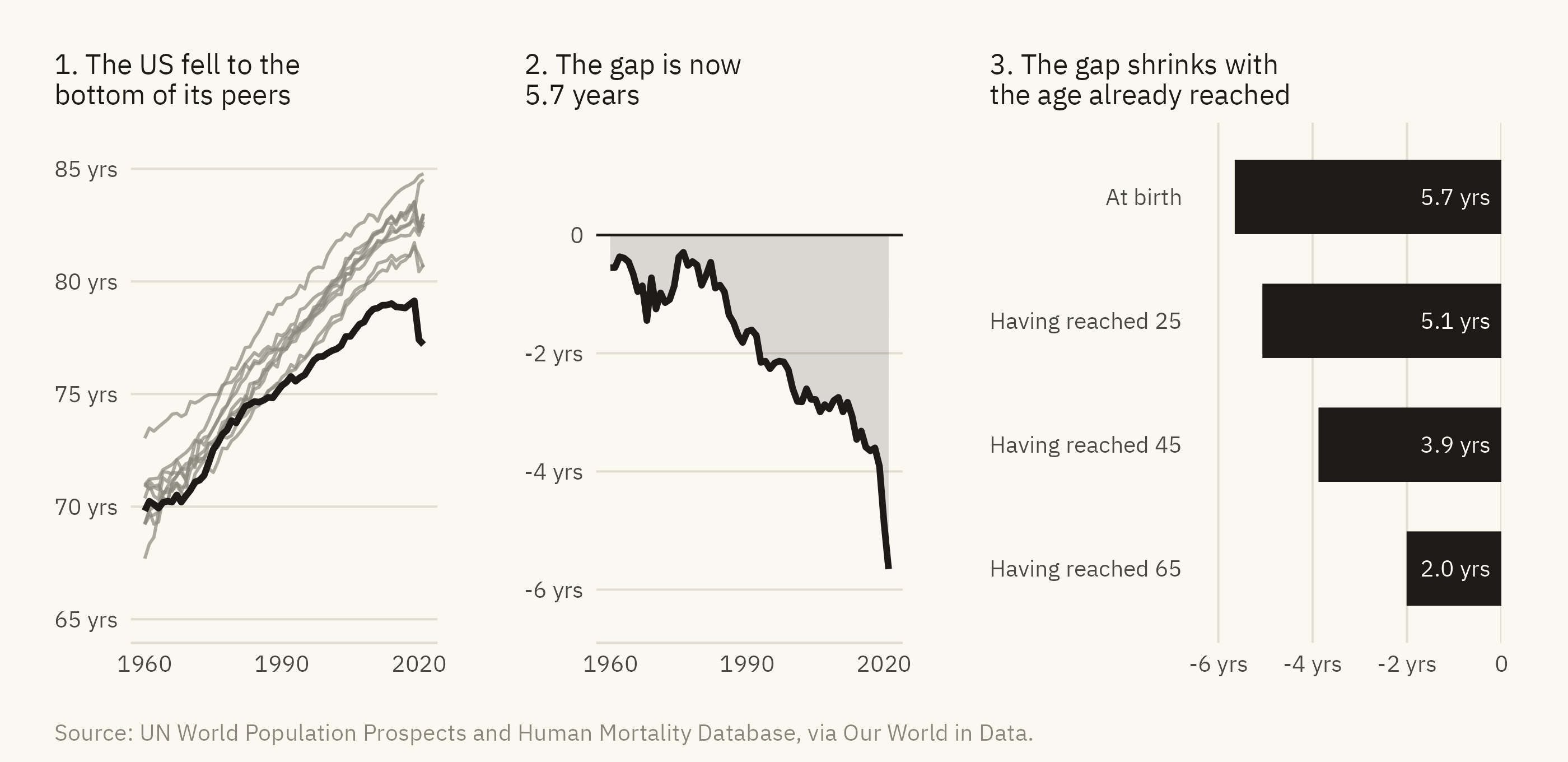
A story from data usually has more than one chart, and the order of the charts is part of the argument. Figure 12.5 contains three panels, each with a title that states a finding.
Show the code
s1 <-ggplot(rich, aes(year, life_expectancy, group = country)) +geom_line(data =filter(rich, country !="United States"), color = mv_ink$mute, linewidth =0.5, alpha =0.7) +geom_line(data =filter(rich, country =="United States"), color =mv_accent(), linewidth =1) +scale_x_continuous(breaks =c(1960, 1990, 2020)) +scale_y_continuous(limits =c(65, 86), breaks =seq(65, 85, 5), labels = \(x) paste0(x, " yrs")) +labs(title ="1. The US fell to the\nbottom of its peers", x =NULL, y =NULL) +theme_mv(base_size =9) + plain_titles2 <-ggplot(gap, aes(year, gap)) +geom_hline(yintercept =0, color = mv_ink$ink, linewidth =0.4) +geom_area(fill =mv_accent(), alpha =0.15) +geom_line(color =mv_accent(), linewidth =1) +scale_x_continuous(breaks =c(1960, 1990, 2020)) +scale_y_continuous(limits =c(-6.5, 1.5), breaks =c(-6, -4, -2, 0), labels = \(x) if_else(x ==0, "0", paste0(x, " yrs"))) +labs(title ="2. The gap is now\n5.7 years", x =NULL, y =NULL) +theme_mv(base_size =9) + plain_titles3 <-ggplot(filter(agl, year ==2021), aes(gap, fct_rev(age))) +geom_col(fill =mv_accent(), width =0.6) +geom_text(aes(x =0, label =sprintf("%.1f yrs", -gap)), hjust =1.15, size =2.6, family =mv_font(), color = mv_ink$canvas) +scale_x_continuous(limits =c(-6.5, 0), expand =expansion(0), breaks =c(-6, -4, -2, 0),labels = \(x) if_else(x ==0, "0", paste0(x, " yrs"))) +labs(title ="3. The gap shrinks with\nthe age already reached", x =NULL, y =NULL) +theme_mv(base_size =9, grid ="x") + plain_titles1 + s2 + s3 +plot_annotation(caption =mv_source(src), theme = cap_theme)
Figure 12.5: The story in three panels. The first shows life expectancy in the United States and its nine peers since 1960. The second shows the gap between the United States and the peer median. The third shows the gap in 2021 by the age already reached. Each panel has one title that states its finding, and the three titles can be read in order as a short paragraph. Source: UN World Population Prospects and Human Mortality Database, via Our World in Data.
I use three panels. The first shows the ten countries and where the United States stands among them. The second shows the size of the gap and when it opened. The third shows how the gap changes with age. What the data cannot show goes in the caption, not in a fourth panel. A reader who reads only the three titles should come away with the finding.
12.8 Step 7: The Checklist
Table 12.1 lists nine questions to answer before publishing a chart. They collect the rules from the earlier chapters, and the second column names the chapter that explains each. A careful reader is likely to ask the same questions of a published chart.
Show the code
tibble::tribble(~Question, ~Chapter,"What is counted, and does the title say so?", "3","Does the chart answer one question, and is it the right question?", "1, 4 to 8","Is the encoding as high on the hierarchy as the data allows?", "2","Do bars start at zero, and do truncated axes say why?", "2, 7","Is the comparison fair, and is the window the full one?", "3, 12","Is the unit of analysis stated, and would the other unit change the story?", "5, 8","Is uncertainty shown where it matters?", "10","Does the title state the finding, with one accent and no legend the chart can do without?", "9","Does the caption say what the data cannot show?", "6, 12") |> knitr::kable()
Table 12.1: The checklist. Nine questions, with the chapter that explains each.
Question
Chapter
What is counted, and does the title say so?
3
Does the chart answer one question, and is it the right question?
1, 4 to 8
Is the encoding as high on the hierarchy as the data allows?
2
Do bars start at zero, and do truncated axes say why?
2, 7
Is the comparison fair, and is the window the full one?
3, 12
Is the unit of analysis stated, and would the other unit change the story?
5, 8
Is uncertainty shown where it matters?
10
Does the title state the finding, with one accent and no legend the chart can do without?
9
Does the caption say what the data cannot show?
6, 12
12.9 Using a Language Model Without Overclaiming
This book was written with the help of a language model. The model drafted code, proposed chart forms, checked arithmetic, and read every chapter against the style rules the author set. Every figure has been rendered from public data by code that is published with the book. Every number in the text has been checked against that output, and the author decided which sentences to keep. The six rules below describe this way of working.
The model drafts. You decide. A model can produce a plausible chart from a vague request in seconds. Treat the result as a first draft from an analyst who has not seen the data before. Chapter 2 listed the common errors in encoding, and Chapter 3 listed the common errors in meaning. Check the draft against both lists.
Put the question in the prompt. “Chart the life expectancy data” usually gets back something like Figure 12.1, with a legend of 236 countries. “Show how far the United States has fallen behind its peers in life expectancy, as a gap over time” usually gets back something close to Figure 12.3. The model draws the chart that the prompt describes, so the prompt has to describe the chart you want.
Check every number. A model will state a correlation, a percentage, or a date with confidence, and sometimes the value is wrong. Compute it yourself and read the documentation for the data. Every number in this book was computed by code run on the data file. None was taken from a model’s answer.
Keep the code. A chart made by clicking in a spreadsheet leaves no record that someone else can check. Neither does a chart that a model hands back as an image. Every figure in this book has its code in the online edition, and Run the Numbers explains how to run it. Anyone who runs the code can check the claim.
Say what the tools did. A reader should know whether a chart came from code the author wrote and can explain, or from a prompt the author typed and a result the author did not inspect. The first paragraph of this section is my disclosure for this book. The copyright page repeats it.
Keep the judgment. Deciding what the reader needs and what the data can support is the author’s job. A model can draft an answer to each of the nine checklist questions and can draft the sentence under the chart. I wrote the final version of each, and I am responsible for them.
ImportantEthics Moment: A Story About People Who Died
A gap of 5.7 years is an average over millions of lives. Behind the gap in Figure 12.4 are Americans who died in their twenties, forties, and sixties when their counterparts in Japan or Sweden did not, and the data do not say what they died of. There are two ways to write about this chart badly. One is to let the reader think the chart explains the deaths. It does not, and a title that states only what the data show avoids the problem. The other is to write about the line as a shape and forget that the shape is made of deaths. A caption that names the measure and the people it counts avoids that problem.
TipTry It Online
Data to Story at viz.marginoferrormedia.com/apps contains the life expectancy data and goes through the seven steps for any country you choose. The app selects a peer group, draws the gap chart, runs the age check, and assembles the three-panel story. It then shows a model’s first-draft caption for the result and asks you to mark every claim the chart does not support.
12.10 Putting It All Together
A story from data follows the seven steps in this chapter. Draw an exploration chart of all the data before choosing a question. Choose a comparison group and state the rule used to choose it. Plot the finding directly, as a difference when the difference is the point. Apply the reading protocol from Chapter 3 to your own chart, and revise the finding if the check requires it. Write the sentence the chart supports, and keep any claim about causes separate from it. Order the charts, usually in three panels, with a title on each that states a finding. Answer the nine questions in the checklist. A language model can draft each step. The author remains responsible for the result of each.
12.11 Further Reading and References
Case, A., and Deaton, A. (2020). Deaths of Despair and the Future of Capitalism. Princeton University Press. A widely cited account of why American life expectancy stalled. The evidence it uses is not in the chapter’s dataset.
Cairo, A. (2019). How Charts Lie. W. W. Norton. The reading protocol applied, at length, to published charts.
Knaflic, C. N. (2015). Storytelling with Data. Wiley. The sequence of setup, finding, and consequence, with worked examples.
National Academies of Sciences, Engineering, and Medicine (2021). High and Rising Mortality Rates Among Working-Age Adults. The National Academies Press. A consensus report on mortality among adults aged 25 to 64 in the United States. Much of the gap in Figure 12.4 arises at these ages.
Roser, M., Ortiz-Ospina, E., and Ritchie, H. (2013, updated 2023). Life expectancy. Our World in Data. The source of the data and an example of documentation for a compiled series.
Woolf, S. H., and Schoomaker, H. (2019). Life expectancy and mortality rates in the United States, 1959–2017. JAMA, 322(20), 1996–2016. A review of the gap and its components in the medical literature.
12.12 Key Terms
Exploration chart. A chart drawn for the author before a question has been chosen. It shows all the data and is not published.
Peer group. The comparison set, chosen by a stated rule and named in the caption.
Gap chart. A chart of the difference between a series and its comparison, computed and plotted as one line.
Period life expectancy. The age a newborn would reach if the death rates of one year applied for that newborn’s whole life. It summarizes the deaths of one year and is not a forecast.
Story sequence. A set of panels, usually three. The first shows the comparison, the second the finding, and the third how the finding varies. The titles can be read in order as a summary.
Disclosure. The statement of what tools did and what the author checked.
12.13 Exercises
Check Your Understanding
Name the four candidate questions discussed under Figure 12.1 and say which one the chapter chose and why.
Why does Figure 12.2 start its axis at 65? Which chapter’s rule allows it, and what does the caption have to do?
What did the age check in Figure 12.4 change about the story, and what did it leave unchanged?
Write the sentence Figure 12.3 supports and one sentence it does not.
Apply the nine-question checklist to Figure 12.5 and record the answer to each.
Apply It
Using ch12-life-expectancy.csv, build the peer comparison for the United Kingdom instead of the United States. Choose and defend a peer group. What is the finding?
Redraw Figure 12.3 with the peer mean in place of the median. Does the story change? Which is the better summary here, and why?
Using ch12-life-expectancy-sex.csv, check whether the American gap differs for women and men. Add the result as a fourth panel to Figure 12.5 and write its title.
Ask a language model for a chart of this data with a vague prompt, then with the question stated. Record the differences against the checklist.
Think Deeper
The chapter chose nine peers by income and data quality. Propose a different rule for the peer group that would be equally defensible, and say how the finding would change.
The section on using a language model says the model drafts and the author decides. Describe a case where the author should not accept the model’s draft even if it is correct.
Write the colophon for a report you have made with these tools, in under a hundred words, following the disclosure rule.