8  Place

8.1 Where

A map is the usual chart for questions about place, such as where children are poor or where rent is high. A map encodes location as position on a surface the reader already knows. Chapter 2 showed that readers judge position more accurately than any other encoding. A map also draws land, and people are not spread evenly over land. When a map colors counties by a rate, large counties with few people take up most of the page. The same data drawn in proportion to population can look quite different.

The case for this chapter is child poverty and housing. The American Community Survey reports the share of children living below the poverty line for every county. The question of where poor children are has two answers. One is the share of children in each place who are poor. The other is the number of poor children in each place. This chapter shows how to put both on the page.

8.2 The Choropleth

A choropleth colors regions by a value. It is the most common kind of thematic map. Figure 8.1 shows one for child poverty by county. It uses a sequential color scale and an equal-area projection. State lines help the reader find places, and a legend explains the colors.

cty <- cty |> mutate(cp_class = cut(child_poverty, breaks = quantile(child_poverty, probs = seq(0, 1, 1/6), na.rm = TRUE),
                                    include.lowest = TRUE, dig.lab = 3))
ggplot(cty) +
  geom_sf(aes(fill = cp_class), color = mv_ink$canvas, linewidth = 0.05) +
  geom_sf(data = states, fill = NA, color = mv_ink$canvas, linewidth = 0.35) +
  scale_fill_manual(values = mv_ramp_seq(6), name = "Child poverty rate (%)", na.value = na_grey,
                    labels = \(x) str_replace_all(x, c("\\[" = "", "\\(" = "", "\\]" = "", "," = " to "))) +
  coord_sf(crs = albers, default_crs = 4326) +
  guides(fill = guide_legend(nrow = 1, label.position = "bottom", title.position = "top")) +
  labs(title = "Child poverty rate by county, 2011 to 2015",
       subtitle = "Share of children under 18 below the poverty line, five-year average",
       caption = mv_source(src)) +
  theme_map()

Figure 8.1: Share of children under 18 living in poverty by county, 2011 to 2015 average. Counties are shaded in six classes by quantile, so each class holds a sixth of counties. The highest rates are in the Deep South, the Mississippi Delta, Appalachia, the Texas border, and reservation counties in the Dakotas and the Southwest. Source: American Community Survey 2011 to 2015; county boundaries from the US Census Bureau.

Four choices went into that map, and the map does not say why any of them was made. They are the projection, the rule for the class breaks, the color ramp, and the decision to map a rate rather than a count. Each could have been made differently. The rest of this chapter covers them in turn.

8.3 Projection

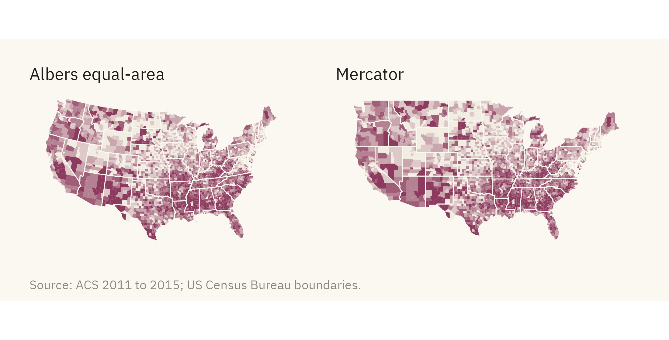
The earth is round and a page is flat, so every projection distorts something. Most web maps use the Mercator projection. It preserves angles and enlarges areas toward the poles. On a Mercator map, Montana looks larger relative to Texas than it is. For a map of the contiguous United States, the standard choice is an Albers equal-area projection. It keeps relative areas correct, and lines of latitude curve slightly on it. Figure 8.2 shows the same map in both projections.

pm <- function(crs, title) {
  ggplot(cty) + geom_sf(aes(fill = cp_class), color = NA) +
    geom_sf(data = states, fill = NA, color = mv_ink$canvas, linewidth = 0.25) +
    scale_fill_manual(values = mv_ramp_seq(6), guide = "none", na.value = na_grey) +
    coord_sf(crs = crs, default_crs = 4326) +
    labs(title = title) + theme_map(base_size = 10) + plain_title
}
pm(albers, "Albers equal-area") + pm(3857, "Mercator") + plot_annotation(caption = mv_source(src), theme = cap_theme)

Figure 8.2: The child poverty map in the Albers equal-area projection (left) and in Mercator (right). Mercator enlarges the northern states. The counties of the northern plains, which have few people and mostly low poverty rates, take up more of the page than their true area. Source: American Community Survey 2011 to 2015.

The difference is small at the scale of the United States and larger on a world map. Mercator draws Greenland about the same size as Africa, although Africa is about fourteen times larger in area. Use an equal-area projection for any map on which the reader will compare areas, which includes every choropleth. Name the projection in the caption.

8.4 Class Breaks

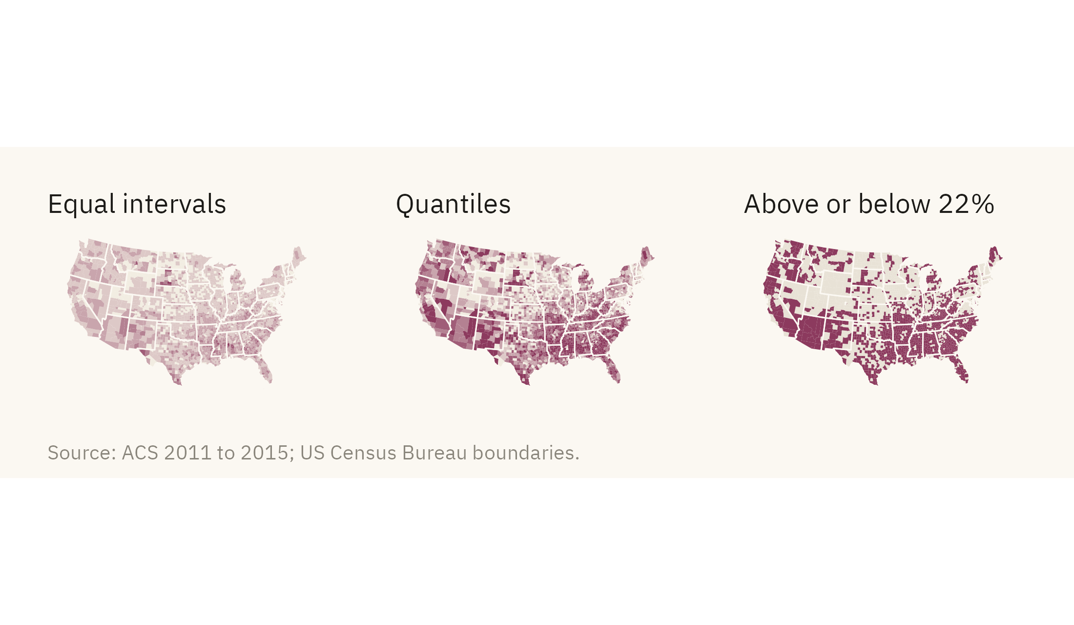
A choropleth turns a continuous rate into a few colors. The rule for cutting the rate into classes changes what the reader sees. Figure 8.3 shows the same rate cut by three rules.

nat_cp <- 22
cty <- cty |> mutate(
  cp_equal = cut(child_poverty, breaks = seq(0, 80, length.out = 7), include.lowest = TRUE),
  cp_two = if_else(child_poverty > nat_cp, "Above the national rate", "At or below"))
pe <- ggplot(cty) + geom_sf(aes(fill = cp_equal), color = NA) +
  geom_sf(data = states, fill = NA, color = mv_ink$canvas, linewidth = 0.25) +
  scale_fill_manual(values = mv_ramp_seq(6), guide = "none", na.value = na_grey) +
  coord_sf(crs = albers, default_crs = 4326) + labs(title = "Equal intervals") + theme_map(base_size = 10) + plain_title
pq <- ggplot(cty) + geom_sf(aes(fill = cp_class), color = NA) +
  geom_sf(data = states, fill = NA, color = mv_ink$canvas, linewidth = 0.25) +
  scale_fill_manual(values = mv_ramp_seq(6), guide = "none", na.value = na_grey) +
  coord_sf(crs = albers, default_crs = 4326) + labs(title = "Quantiles") + theme_map(base_size = 10) + plain_title
pt <- ggplot(cty) + geom_sf(aes(fill = cp_two), color = NA) +
  geom_sf(data = states, fill = NA, color = mv_ink$canvas, linewidth = 0.25) +
  scale_fill_manual(values = c(`Above the national rate` = mv_accent(), `At or below` = "#E8E2D6"), guide = "none", na.value = na_grey) +
  coord_sf(crs = albers, default_crs = 4326) + labs(title = "Above or below 22%") + theme_map(base_size = 10) + plain_title
pe + pq + pt + plot_annotation(caption = mv_source(src), theme = cap_theme)

Figure 8.3: Child poverty by county with three rules for class breaks. Equal intervals cut the range into even steps, and most counties fall in the first two classes. Quantiles put a sixth of counties in each class and show the full spread. A single break at the national rate of 22 percent shows one comparison only. Source: American Community Survey 2011 to 2015.

With equal intervals, each class covers the same width of the rate, but the pattern is hard to see. Ten counties above 60 percent widen the range, so two thirds of counties fall in the two lightest classes. With quantiles, the pattern is visible, but the classes cover unequal widths. The darkest class runs from 32 to 72 percent. A single break at a meaningful threshold, here the national rate of 22 percent, shows less detail. The reader can then state the comparison in one sentence. Choose the breaks for the question and print them in the legend. Most software uses equal intervals unless you choose otherwise.

8.5 Rate or Count

The maps so far show a rate. A reader who wants to know where poor children live needs a map of counts. A choropleth of counts tends to mislead, because counties with large populations have large counts of everything. The standard form for a count on a map is a proportional symbol. It places a circle at each county’s center and sizes the circle by the number. Figure 8.4 shows this for children in poverty.

cent <- cty |> filter(!is.na(child_poverty)) |>
  mutate(poor_children = pop * 0.23 * child_poverty / 100) |>
  st_point_on_surface() |>
  st_transform(albers)
big <- cent |> slice_max(poor_children, n = 5) |> mutate(label = str_remove(county, " County"),
                                                         x = st_coordinates(geometry)[, 1], y = st_coordinates(geometry)[, 2]) |> st_drop_geometry()
ggplot() +
  geom_sf(data = states, fill = "#F2EDE2", color = mv_ink$canvas, linewidth = 0.35) +
  geom_sf(data = cent, aes(size = poor_children), color = mv_accent(), alpha = 0.45, shape = 16) +
  geom_text_repel(data = big, aes(x, y, label = label),
                  size = 3, family = mv_font(), color = mv_ink$ink, bg.color = mv_ink$canvas, bg.r = 0.12,
                  min.segment.length = 0, segment.color = mv_ink$ink, box.padding = 0.8, point.padding = 1.5, seed = 8) +
  scale_size_area(max_size = 16, breaks = c(25000, 100000, 300000), labels = label_comma(), name = "Children in poverty") +
  coord_sf(crs = albers) +
  labs(title = "Number of children in poverty by county,\n2011 to 2015",
       subtitle = "Estimated number of children under 18\nbelow the poverty line",
       caption = "Source: ACS 2011 to 2015; US Census Bureau boundaries.\nChildren estimated as 23 percent of county population.") +
  theme_map() + theme(legend.key.height = unit(1.4, "lines"))

Figure 8.4: Number of children in poverty by county, one circle per county sized by the count. The five largest counts are labeled. Los Angeles County alone has more poor children than 42 of the 48 contiguous states. Most of the large circles are in metropolitan counties, which sit in the middle classes of the rate map. Source: American Community Survey 2011 to 2015.

Compare Figure 8.1 with Figure 8.4. The rate map shows the highest shares in the South and on reservations. The count map shows the largest numbers in the cities. Both are accurate. A policy based on the rate map would send help to where the share of poor children is highest. A policy based on the count map would send help to where the number of poor children is largest. When a report includes only one of the two maps, the reader sees only one of the two answers.

8.6 Land Is Not People

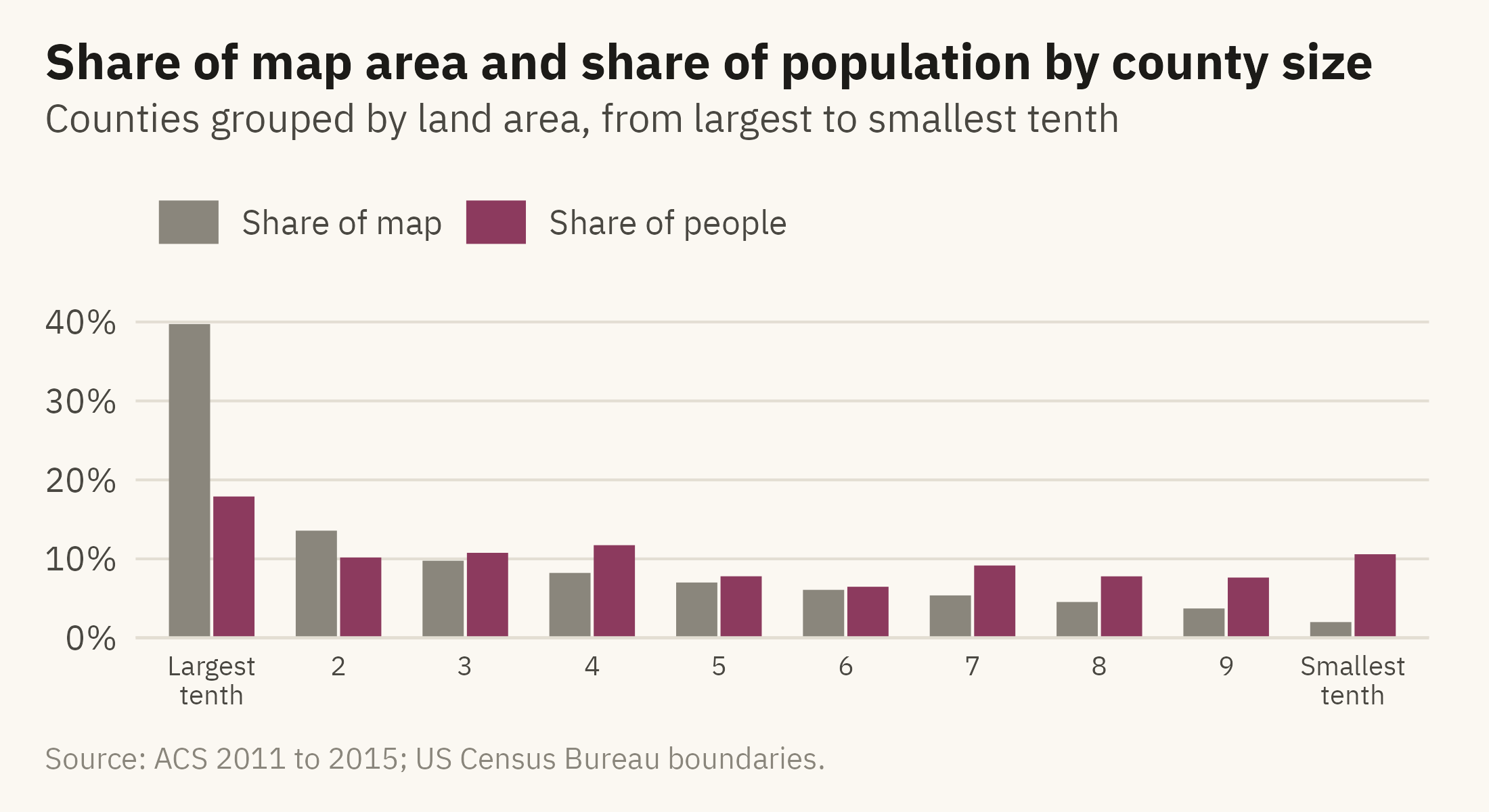
The main problem with a choropleth is that it weights by land area. Figure 8.5 shows the size of the problem with a bar chart. The 100 largest counties by area hold 10 percent of the population and cover 22 percent of the map.

cty_area <- cty |> mutate(area = as.numeric(st_area(st_transform(geometry, albers)))) |> st_drop_geometry() |>
  filter(!is.na(pop)) |> arrange(desc(area)) |>
  mutate(decile = ntile(area, 10), decile = 11 - decile) |>
  group_by(decile) |> summarise(area = sum(area), pop = sum(pop), .groups = "drop") |>
  mutate(`Share of map` = area / sum(area), `Share of people` = pop / sum(pop)) |>
  pivot_longer(c(`Share of map`, `Share of people`), names_to = "what", values_to = "share") |>
  mutate(decile = factor(decile, labels = c("Largest\ntenth", paste0(2:9), "Smallest\ntenth")))
ggplot(cty_area, aes(decile, share, fill = what)) +
  geom_col(position = position_dodge(width = 0.7), width = 0.65) +
  scale_fill_manual(values = c(`Share of map` = mv_ink$mute, `Share of people` = mv_accent()), name = NULL) +
  scale_y_continuous(labels = label_percent(), expand = expansion(mult = c(0, 0.05))) +
  labs(title = "Share of map area and share of population by county size",
       subtitle = "Counties grouped by land area, from largest to smallest tenth",
       x = NULL, y = NULL, caption = mv_source(src)) +
  theme_mv() + theme(axis.text.x = element_text(size = rel(0.8), lineheight = 0.9))

Figure 8.5: Counties sorted by land area, grouped into ten bins of about 310 counties each. The largest tenth of counties by area holds 18 percent of the population and covers 40 percent of the map. The smallest tenth holds 11 percent of the population on 2 percent of the land. Source: American Community Survey 2011 to 2015; areas from county boundaries.

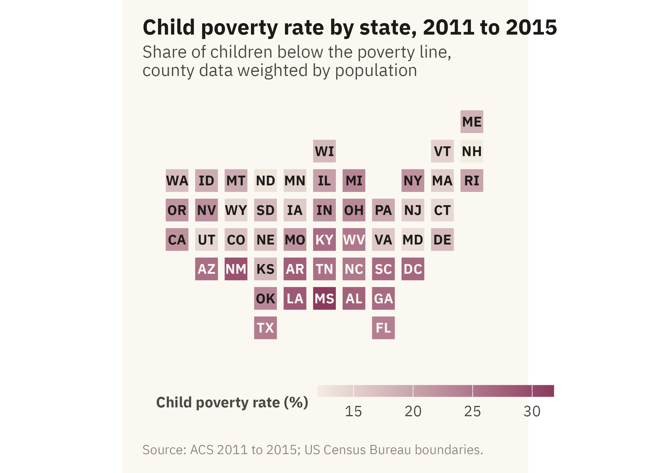
Three methods address the problem. The first is to map a rate and pair it with a count, as above. The second is to map people rather than land, with a symbol map or a dot density map. The third is to drop geographic shape and draw a tile grid. In a tile grid, every state is the same size and is placed near its true position. Figure 8.6 shows child poverty by state this way.

grid <- tribble(
  ~st, ~col, ~row,
  "ME",11,1, "WI",6,2, "VT",10,2, "NH",11,2, "WA",1,3, "ID",2,3, "MT",3,3, "ND",4,3, "MN",5,3, "IL",6,3, "MI",7,3, "NY",9,3, "MA",10,3, "RI",11,3,
  "OR",1,4, "NV",2,4, "WY",3,4, "SD",4,4, "IA",5,4, "IN",6,4, "OH",7,4, "PA",8,4, "NJ",9,4, "CT",10,4,
  "CA",1,5, "UT",2,5, "CO",3,5, "NE",4,5, "MO",5,5, "KY",6,5, "WV",7,5, "VA",8,5, "MD",9,5, "DE",10,5,
  "AZ",2,6, "NM",3,6, "KS",4,6, "AR",5,6, "TN",6,6, "NC",7,6, "SC",8,6, "DC",9,6,
  "OK",4,7, "LA",5,7, "MS",6,7, "AL",7,7, "GA",8,7, "TX",4,8, "FL",8,8)
abbr <- c(setNames(state.abb, state.name), "District of Columbia" = "DC")
st_cp <- acs |> mutate(st = abbr[state]) |> filter(!is.na(st), !is.na(child_poverty)) |>
  group_by(st) |> summarise(cp = weighted.mean(child_poverty, pop), .groups = "drop") |>
  right_join(grid, by = "st")
ggplot(st_cp, aes(col, -row, fill = cp)) +
  geom_tile(color = mv_ink$canvas, linewidth = 1.5, width = 0.95, height = 0.95) +
  geom_text(aes(label = st, color = cp > 24), size = 3, family = mv_font(), fontface = "bold") +
  scale_color_manual(values = c(`TRUE` = mv_ink$canvas, `FALSE` = mv_ink$ink), guide = "none") +
  scale_fill_gradientn(colors = mv_ramp_seq(9), name = "Child poverty rate (%)") +
  coord_equal() +
  labs(title = "Child poverty rate by state, 2011 to 2015",
       subtitle = "Share of children below the poverty line,\ncounty data weighted by population",
       caption = mv_source(src)) +
  theme_map() + theme(legend.key.width = unit(2, "lines"))

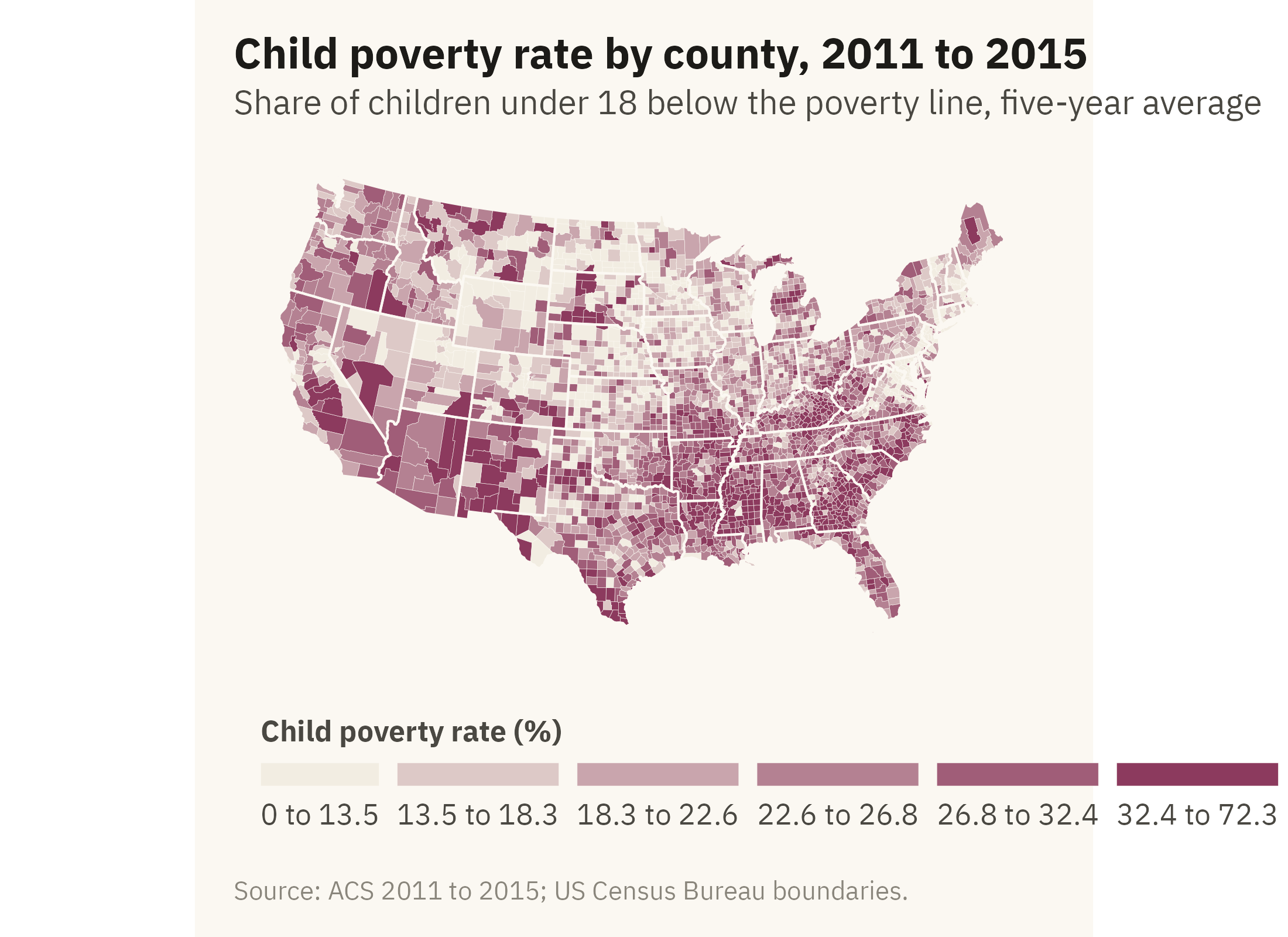
Figure 8.6: Child poverty rate by state on a tile grid. Each state is one square, placed near its geographic position. In the grid, Rhode Island and Texas have the same space, so the small Northeastern states are easy to read. State shapes and some adjacencies are lost. Source: American Community Survey 2011 to 2015, counties aggregated with population weights.

8.7 Points on a Map

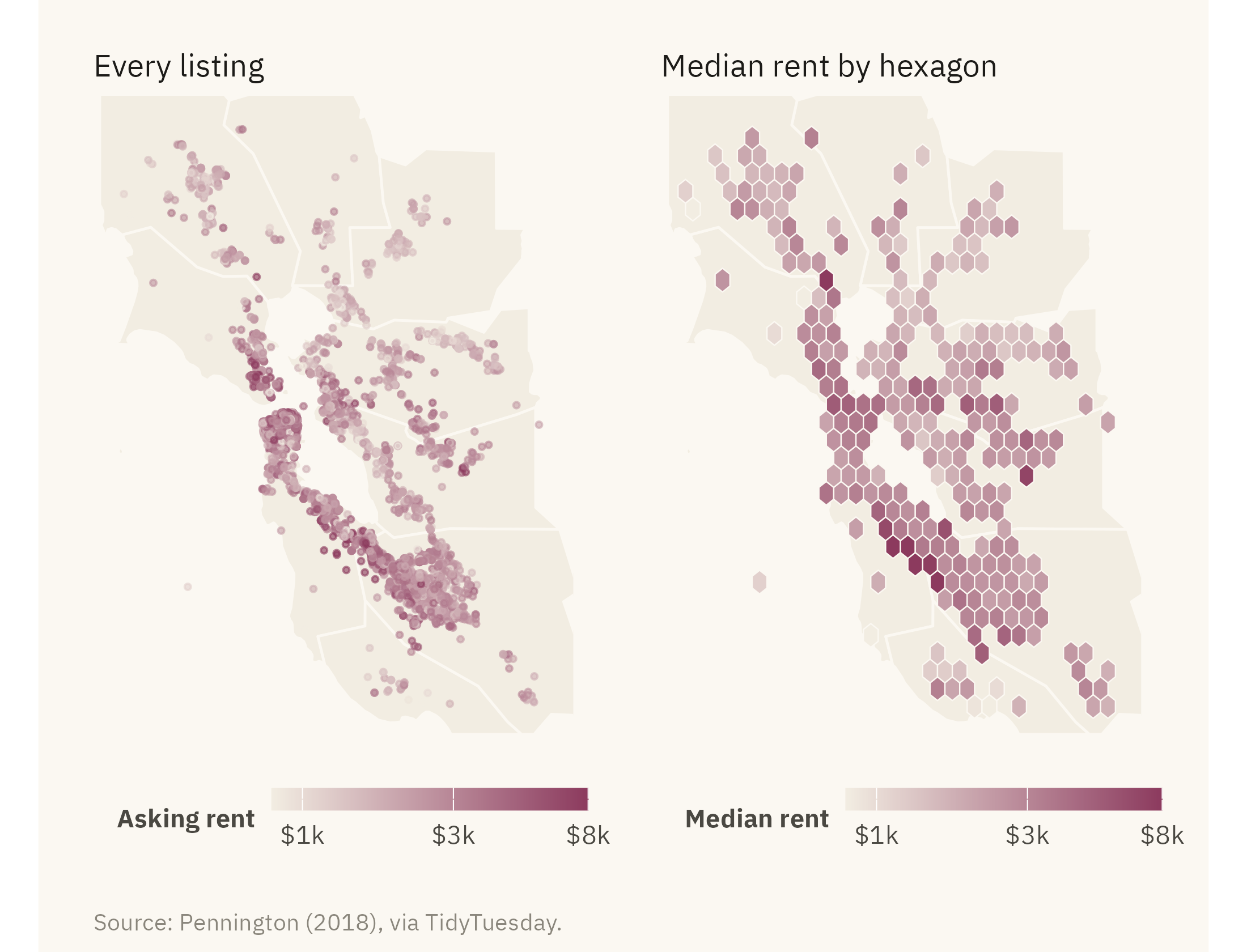
Not every spatial question is about regions. The Bay Area rental data in Figure 8.7 is a set of listings, each with coordinates. The question is where rent is high within one metropolitan area. A point for each listing can answer it. With thousands of listings, the points overlap and cover each other. One remedy is to group the points into bins.

bay_fips <- c("06001", "06013", "06041", "06055", "06075", "06081", "06085", "06087", "06095", "06097")
bay <- co |> filter(fips %in% bay_fips)
r2 <- rent |> filter(lon > -123, lon < -121.5, lat > 37, lat < 38.6)
pts <- ggplot() +
  geom_sf(data = bay, fill = "#F2EDE2", color = mv_ink$canvas, linewidth = 0.4) +
  geom_point(data = r2, aes(lon, lat, color = price), size = 0.6, alpha = 0.6) +
  scale_color_gradientn(colors = mv_ramp_seq(9), trans = "log10", limits = c(800, 8000), oob = scales::squish,
                        breaks = c(1000, 3000, 8000), labels = c("$1k", "$3k", "$8k"), name = "Asking rent") +
  coord_sf(xlim = c(-123, -121.5), ylim = c(37, 38.6), default_crs = 4326) +
  labs(title = "Every listing") + theme_map(base_size = 10) + plain_title + theme(legend.key.width = unit(1.4, "lines"))
hx <- ggplot() +
  geom_sf(data = bay, fill = "#F2EDE2", color = mv_ink$canvas, linewidth = 0.4) +
  stat_summary_hex(data = r2, aes(lon, lat, z = price), fun = median, bins = 28, color = mv_ink$canvas, linewidth = 0.2) +
  scale_fill_gradientn(colors = mv_ramp_seq(9), trans = "log10", limits = c(800, 8000), oob = scales::squish,
                       breaks = c(1000, 3000, 8000), labels = c("$1k", "$3k", "$8k"), name = "Median rent") +
  coord_sf(xlim = c(-123, -121.5), ylim = c(37, 38.6), default_crs = 4326) +
  labs(title = "Median rent by hexagon") + theme_map(base_size = 10) + plain_title + theme(legend.key.width = unit(1.4, "lines"))
pts + hx + plot_annotation(caption = mv_source("Pennington (2018), via TidyTuesday"), theme = cap_theme)

Figure 8.7: Craigslist rental listings in the San Francisco Bay Area with coordinates, 2001 to 2018. Left, every listing as a point colored by asking rent. Right, listings grouped into hexagons, each shaded by its median rent. The hexagons do not overlap, and their shading shows that rent falls with distance from San Francisco and the Peninsula. Source: Pennington (2018), via TidyTuesday.

The hexagon map is a choropleth whose regions are set by the analyst rather than by political boundaries. The hexagons are equal in area, so the land-area problem does not arise. Their size can be set to match the density of the data. Most readers have not seen hexagon maps before, so the caption and legend need to explain them. The color uses a log scale here for the reason given in Chapter 5. Rents span a tenfold range, and on a linear ramp most of the colors would go to the few highest rents.

8.8 Two Maps: Change

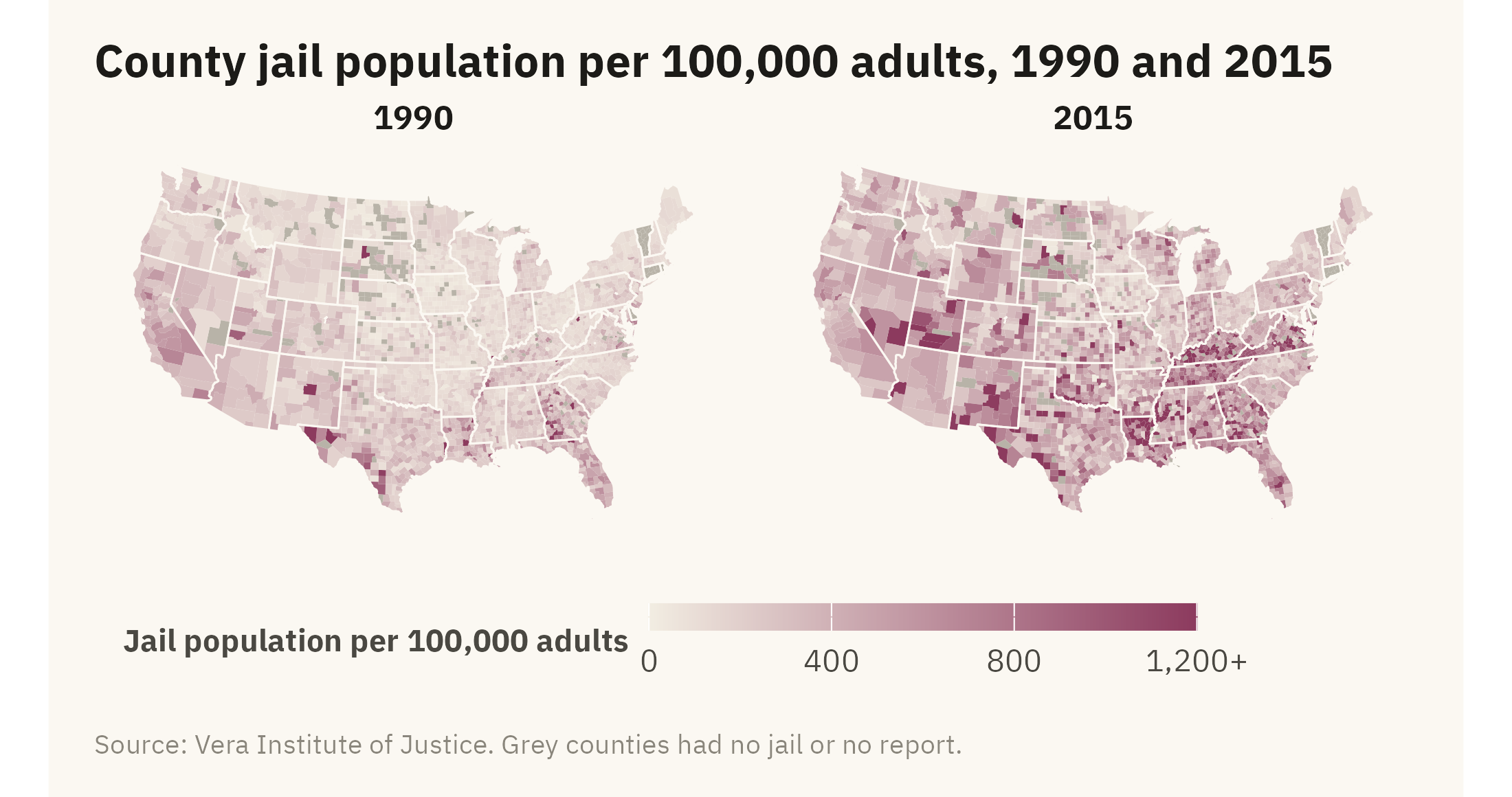
A map shows one moment in time. To show change, you need either two maps or a map of the difference. Figure 8.8 draws the county jail rate from Chapter 7 in 1990 and 2015 as small multiples on one color scale.

jl <- cty |> select(fips, jail_rate_1990, jail_rate_2015) |>
  pivot_longer(c(jail_rate_1990, jail_rate_2015), names_to = "year", values_to = "rate", names_prefix = "jail_rate_") |>
  mutate(rate = if_else(rate <= 0, NA, rate), rate_c = pmin(rate, 1200))
ggplot(jl) +
  geom_sf(aes(fill = rate_c), color = NA) +
  geom_sf(data = states, fill = NA, color = mv_ink$canvas, linewidth = 0.25) +
  facet_wrap(~ year) +
  scale_fill_gradientn(colors = mv_ramp_seq(9), na.value = na_grey, limits = c(0, 1200),
                       breaks = c(0, 400, 800, 1200), labels = c("0", "400", "800", "1,200+"), name = "Jail population per 100,000 adults") +
  coord_sf(crs = albers, default_crs = 4326) +
  labs(title = "County jail population per 100,000 adults, 1990 and 2015", caption = mv_source("Vera Institute of Justice", "grey counties had no jail or no report")) +
  theme_map(base_size = 10) + theme(strip.text = element_text(hjust = 0.5), legend.key.width = unit(2, "lines"))

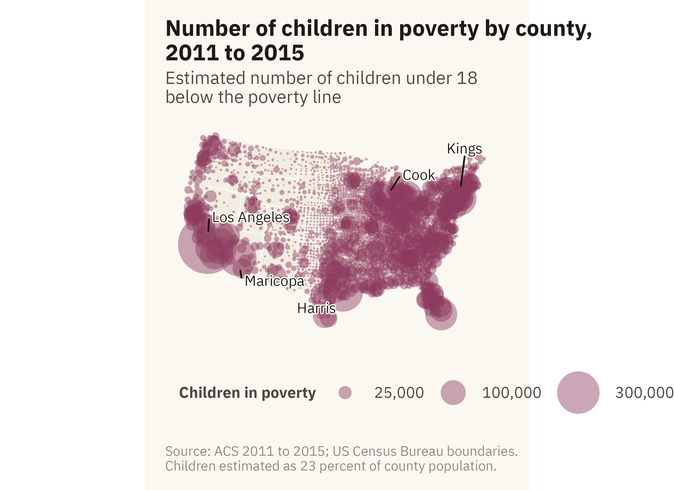
Figure 8.8: County jail population per 100,000 adults in 1990 and 2015 on the same color scale. Rates rose across the South over the period. The rural counties of Kentucky, Virginia, Tennessee, and Louisiana rose most. Counties with no jail or no report are grey, 187 in 1990 and 175 in 2015. Source: Vera Institute of Justice, Incarceration Trends; boundaries from the US Census Bureau.

With two maps on one scale, the reader has to compare shades across panels. Chapter 2 ranked comparison of color intensity near the bottom of the hierarchy. A third map of the difference, on a diverging scale centered at zero, would show the change directly but not the levels. The complete version is a pair of figures, with levels as small multiples and change on its own map, each labeled. When there is room for only one, keep the one that answers the question asked.

ImportantEthics Moment: The County Line

A county is a unit of government, and its population can be anything from a few dozen people to ten million. Oglala Lakota County in South Dakota covers the Pine Ridge Reservation. On Figure 8.1 it is in the darkest class, with a child poverty rate of 62 percent. Los Angeles County has more poor children than 42 of the 48 contiguous states and sits in the fourth of six classes, at 26 percent. Both maps are accurate. A reader who sees only the rate map may conclude that child poverty is rural and Native. A reader who sees only the count map may conclude that it is urban. Each conclusion is incomplete. A rate map needs the count map beside it, and a count map needs the rate map. If there is no room, add a sentence that says what the map leaves out.

TipTry It Online

Same Place, Four Maps at viz.marginoferrormedia.com/apps holds the county data. Choose a variable and switch among a quantile choropleth, an equal-interval choropleth, proportional symbols, and the state tile grid. A slider changes the number of classes, and a toggle switches the projection. Try to find a class rule under which the Deep South looks no different from the rest of the country. Such a rule exists. Print the class rule in the legend so the reader can check it.

WarningAI Reality Check: Generated Maps

Errors in generated maps are often hard to notice. A common first draft is a choropleth of counts, in Mercator, with equal intervals and a rainbow color ramp. Each of those four choices is covered in this chapter or in Chapter 2. The result still looks like a map, and Monmonier (2018) notes that readers tend to accept a map as accurate. A model is unlikely to point out that Los Angeles County has ten million people and Loving County, Texas, has about a hundred. It is also unlikely to warn that the map weights by land area rather than by population.

Ask for a rate, an equal-area projection, quantile or threshold breaks, and a single-hue ramp. Ask for the count as symbols beside it. Also ask the model which counties have no data. Software fills every polygon with a color whether or not data exist for it. A grey county for missing data and a white county for a low value mean different things. The legend should say which is which.

8.9 Putting It All Together

A map encodes place as position on a surface the reader already knows, and it weights by land area. Choose an equal-area projection and name it in the caption. Choose class breaks for the question and print them in the legend. Map rates as colors and counts as symbols. Show both when the question is about people. Use a tile grid or a symbol map when the land-area weighting misleads. Group points into bins when they overlap. Show change as two maps on one scale or as a map of the difference, not as one map with a claim about change in its title.

8.10 Looking Ahead

Part III moves from choosing a chart to finishing one. Chapter 9 covers color, type, and annotation. These three decisions affect whether a reader can read a correct chart with ease. The case is public attitudes toward immigration. The chart there has to show a pattern in opinion without taking a side.

8.11 Further Reading and References

Brewer, C. A. (2016). Designing Better Maps: A Guide for GIS Users, 2nd edition. Esri Press. The standard reference for class breaks, color, and projection in thematic maps.

Field, K. (2018). Cartography. Esri Press. A broad and opinionated survey of map design with many examples of the problems in this chapter.

Monmonier, M. (2018). How to Lie with Maps, 3rd edition. University of Chicago Press. The map equivalent of Huff, and the source of much of the thinking on choropleths and projections here.

Pennington, K. (2018). Bay Area Craigslist Rental Housing Posts, 2000 to 2018. Dataset. The rental listings used in Figure 8.7.

Tobler, W. (1973). Choropleth maps without class intervals? Geographical Analysis, 5(3), 262–265. The argument for unclassed choropleths, which this chapter does not follow, and why.

8.12 Key Terms

Choropleth. Regions colored by a value. The most common thematic map. It weights by land area.

Equal-area projection. A way of flattening the earth that keeps relative areas correct. Albers for the United States.

Class breaks. The rule for cutting a continuous value into colors. Equal intervals, quantiles, or thresholds.

Proportional symbol map. A circle at each place sized by a count. The standard form for counts on a map.

Tile grid map. Every region the same size, placed near its position. Drops shape so that every region has equal space.

Hexagonal binning. Grouping points into equal-area hexagons and shading each by a summary such as the median.

8.13 Exercises

Check Your Understanding

1. State the four hidden choices in Figure 8.1 and what each one could have been instead.
2. Why does a choropleth of counts mislead? What does a proportional symbol map do differently?
3. In Figure 8.3, which class rule would you choose for a report on where to send aid, and which for a report on how unequal the country is?
4. Figure 8.5 shows that the largest tenth of counties covers 40 percent of the map. What does that imply about what a reader sees first in Figure 8.1?
5. What does a tile grid give up, and when is that cost worth paying?

Apply It

6. Using ch08-county-acs-2015.csv and the county boundaries, map the unemployment rate with quantile breaks and then with a single break at the national rate. Write the one sentence each map supports.
7. Draw a proportional symbol map of total population and overlay it on the child poverty choropleth. Describe where the two disagree.
8. Build a hexagon map of median rent for one-bedroom listings only. Does the pattern change from Figure 8.7?
9. Make a map of the change in jail rate from 1990 to 2015 on a diverging scale centered at zero. Compare it with Figure 8.8 and say which is easier to read and which shows the levels more accurately.

Think Deeper

10. The chapter maps the contiguous 48 states and omits Alaska and Hawaii. What does the omission cost, and how would you add them without distorting the rest?
11. A county has 100 residents and a child poverty rate of 50 percent. Propose a rule for how such counties should be shown on a choropleth, and apply it to Figure 8.1.
12. The Ethics Moment says the rate map and the count map each leave out part of the picture. Design a single figure that shows both without a dual encoding, and sketch its caption.