On the evening of January 27, 1986, engineers at Morton Thiokol held a teleconference with NASA. Thiokol built the solid rocket boosters for the Space Shuttle. The forecast for the next morning’s launch at Cape Canaveral was 26 to 29 degrees Fahrenheit. No earlier launch had taken place at a temperature near that. Several Thiokol engineers were concerned, because the rubber O-rings that sealed the joints between booster segments became stiff in the cold, and O-ring damage had been found after earlier flights.
The engineers argued against launching. They had prepared charts for the call. The charts listed O-ring damage for each flight, with the flight identified by its serial number and the temperature noted in a column. Someone who already understood the concern could find the relationship between temperature and damage in those charts. Someone seeing them for the first time, on a tense call late at night, could not. After several hours of discussion, Thiokol’s managers overruled their engineers and recommended launch. Seventy-three seconds after liftoff the next morning, an O-ring on the right booster failed. The orbiter broke apart, and seven people died.
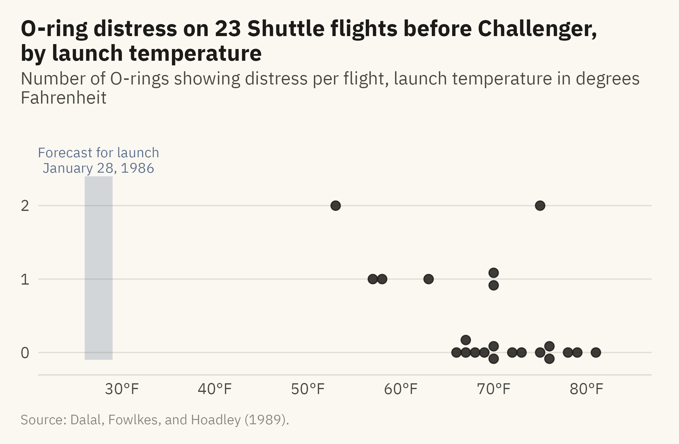
In Visual Explanations (1997), Edward Tufte redrew the engineers’ data as a single chart, with damage on the vertical axis and temperature on the horizontal axis. Each earlier flight is a point, and the forecast launch temperature is marked to the left of every point. Figure 2.1 is that chart, drawn from the data the engineers had that night.
Show the code
orings_sp <- orings |>group_by(temp_f, distress) |>mutate(y = distress + (row_number() - (n() +1) /2) *0.17) |>ungroup()ggplot(orings_sp, aes(temp_f, y)) +annotate("rect", xmin =26, xmax =29, ymin =-0.1, ymax =2.4, fill =mv_accent(), alpha =0.25) +annotate("text", x =27.5, y =2.45, label ="Forecast for launch\nJanuary 28, 1986", vjust =0,size =2.9, family =mv_font(), color =mv_accent(), lineheight =0.9) +geom_point(size =2.2, color = mv_ink$ink, alpha =0.85) +scale_x_continuous(limits =c(24, 84), breaks =seq(30, 80, 10),labels = \(x) paste0(x, "°F")) +scale_y_continuous(breaks =0:2, limits =c(-0.15, 2.95)) +labs(title ="O-ring distress on 23 Shuttle flights before Challenger, by launch temperature",subtitle ="Number of O-rings showing distress per flight, launch temperature in degrees Fahrenheit",x =NULL, y =NULL, caption =mv_source("Dalal, Fowlkes, and Hoadley (1989)")) +theme_mv()
Figure 2.1: O-ring distress on the 23 Space Shuttle flights before Challenger, by temperature at launch. Every flight below 65 degrees showed damage. Flights that share a temperature are stacked so each is visible. The forecast for January 28, 1986 is marked. Source: Dalal, Fowlkes, and Hoadley (1989).
Tufte did not claim that a better chart would have saved the crew. The decision failed for many reasons, and the engineers who were on the call have objected to any account that blames a slide. The case supports a narrower claim. The engineers had the data that supported their argument, but they did not have a form of the data in which the relationship could be seen without study. When temperature is placed on the horizontal axis, as in Figure 2.1, the relationship between cold and damage can be seen in a few seconds.
This chapter explains why some forms of a chart can be read in a few seconds and others cannot. The visual system has rules and limits, and most of them have been measured in experiments. A designer who knows those results can use them. A designer who does not know them is guessing.
2.2 The Case: Air We Cannot See
The subject of this chapter is fine particulate matter, called PM2.5. These are particles of dust and soot small enough to pass from the lungs into the blood. In 2021, the World Health Organization set its guideline for annual exposure at 5 micrograms per cubic meter of air. The World Bank publishes a population-weighted estimate of exposure for every country, and the series used here ends in 2017. In that year, every one of the 191 countries with data was above the guideline. A quarter of them were above 35 micrograms, which is the loosest of the WHO’s interim targets.
Air pollution is a useful case for a chapter on perception because the harm cannot be seen and the numbers are hard to interpret. Most readers have no sense of what “90 micrograms per cubic meter” for India means, or how it compares with “7” for the United States. The charts in this chapter have to give the reader that sense. Each demonstration uses this data, and the chapter ends with a chart that combines the lessons.
2.3 Two Kinds of Looking
Vision carries more information per second than the other senses combined, but the visual system does not process everything at the same speed. Research since the 1970s, much of it from Anne Treisman’s laboratory, describes visual processing as two stages.
The first stage is preattentive processing. It is fast, parallel, and automatic. It covers the whole visual field in about a quarter of a second, before attention is directed anywhere. Certain features are detected at this stage with no effort. Color, position, size, orientation, and motion are among them. The second stage is attentive processing. It is slow and serial, and it examines one element at a time.
This has a direct consequence for chart design. If the message of a chart is carried by a feature that is detected preattentively, a reader will see it before deciding to look for it. If the message depends on a feature that requires attentive processing, the reader has to search for it, and many readers will not. The list of preattentive features is short. It includes position, length, slope, orientation, size, shape, hue, intensity, motion, and enclosure. A well-made chart uses one or two of these for the data and reserves the rest for labels.
Show the code
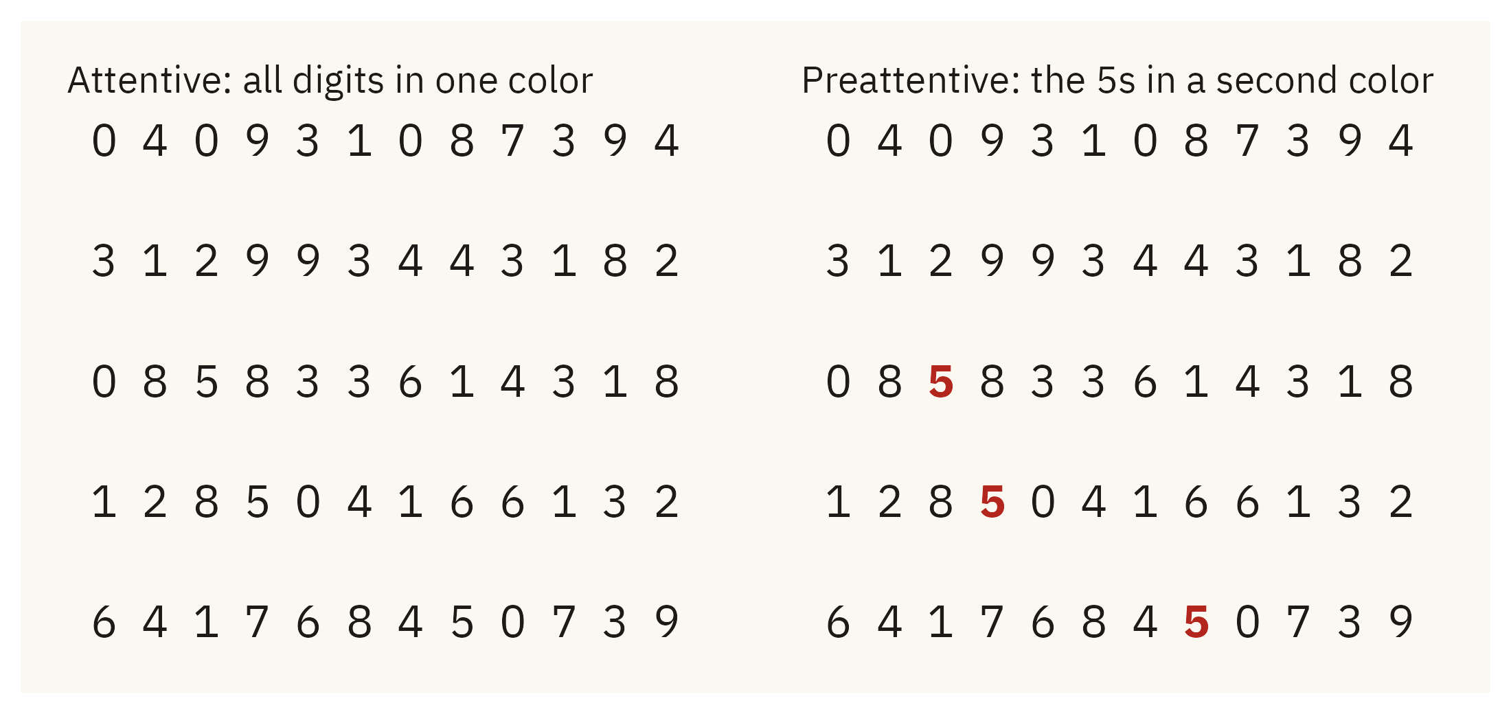
set.seed(42)grid <-expand_grid(row =1:5, col =1:12) |>mutate(digit =sample(c(0:4, 6:9), n(), replace =TRUE))grid$digit[c(27, 40, 56)] <-5grid <- grid |>mutate(is5 = digit ==5)p_plain <-ggplot(grid, aes(col, -row, label = digit)) +geom_text(family =mv_font(), size =4.2, color = mv_ink$ink) +labs(title ="Attentive: all digits in one color") +theme_mv_blank(base_size =10) +theme(plot.title =element_text(size =rel(1), face ="plain"))p_pop <-ggplot(grid, aes(col, -row, label = digit, color = is5)) +geom_text(family =mv_font(), size =4.2, fontface =ifelse(grid$is5, "bold", "plain")) +scale_color_manual(values =c(`FALSE`= mv_ink$ink, `TRUE`="#B3261E"), guide ="none") +labs(title ="Preattentive: the 5s in a second color") +theme_mv_blank(base_size =10) +theme(plot.title =element_text(size =rel(1), face ="plain"))p_plain + p_pop
Figure 2.2: The same digits in the same positions, drawn twice. On the left, all digits are one color, and a reader finds the 5s one digit at a time. On the right, the 5s are in a second color. A reader can see them at once, because color is a preattentive feature.
2.4 The Hierarchy of Encodings
Preattentive features differ in how accurately they can be judged. In 1984, William Cleveland and Robert McGill at Bell Labs asked participants to compare quantities that had been encoded in different ways. Some comparisons were between two bars, which is a comparison of lengths. Some were between two pie slices, which is a comparison of angles. Some were between two segments of a stacked bar, which do not share a baseline. Some were between two shaded cells, which is a comparison of intensities. For each encoding, Cleveland and McGill measured the error in the participants’ judgments.
Position along a common scale was judged most accurately. Length along a common baseline came next. Slope and angle were judged less accurately, and area less accurately still. Color intensity and volume had the largest errors, and the errors grew as the two quantities moved further apart. The result has been replicated many times, including by Jeffrey Heer and Michael Bostock in 2010 with thousands of online participants. The working version of the Cleveland and McGill hierarchy, from most accurate to least accurate, is:
Position along a common scale (a dot plot, a scatter plot)
Position along non-aligned scales (small multiples with separate baselines)
Length (a bar chart)
Slope (a line chart)
Angle (a pie chart)
Area (a bubble chart, a treemap)
Color intensity (a heatmap, a shaded map)
Color hue (a categorical map)
Volume (a chart with a 3D effect)
The ranking concerns accuracy when a reader compares quantities. It does not say which chart looks better, and it does not say that hue is bad. Hue is suitable for categories and unsuitable for ordered values. The next three sections apply the hierarchy to the air pollution data.
Angle Against Length
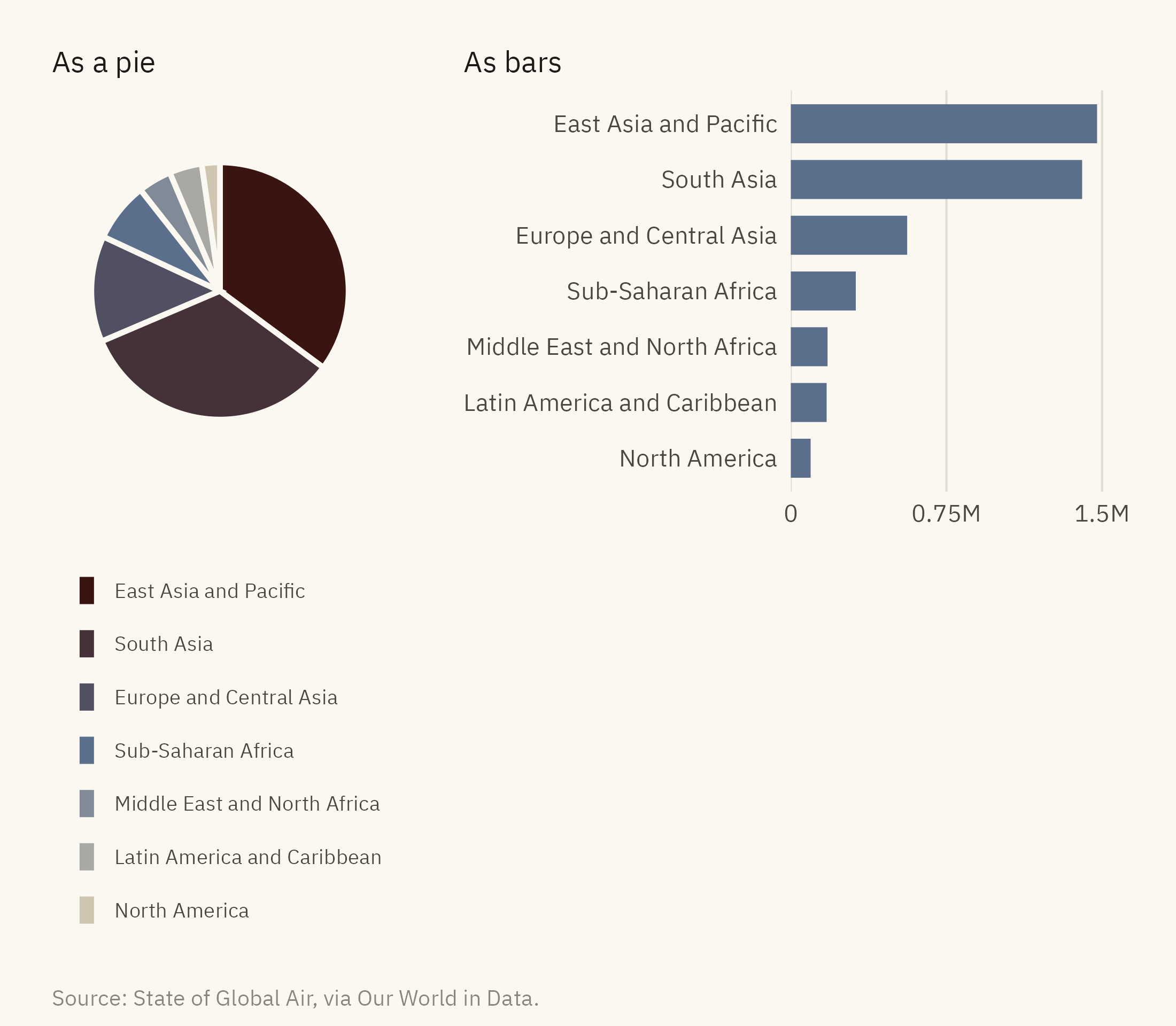
Figure 2.3 shows deaths attributed to outdoor PM2.5 in 2015 by world region, first as a pie chart and then as a bar chart. Look at the pie first and try to decide whether East Asia or South Asia is larger, and how much larger Europe is than Sub-Saharan Africa. Then try the same comparisons with the bars.
Show the code
reg <- deaths |>filter(year ==2015, !is.na(region)) |>group_by(region) |>summarise(d =sum(deaths_ambient_pm25, na.rm =TRUE), .groups ="drop") |>mutate(region =str_replace(region, " & ", " and "),region =fct_reorder(region, d))pie <-ggplot(reg, aes(x =1, y = d, fill = region)) +geom_col(color = mv_ink$canvas, linewidth =0.9) +coord_polar(theta ="y") +scale_fill_manual(values =colorRampPalette(c("#CFC6B2", mv_accent(), "#3A1410"))(7)) +labs(fill =NULL, title ="As a pie") +guides(fill =guide_legend(ncol =1, reverse =TRUE)) +theme_mv_blank(base_size =10) +theme(legend.position ="bottom", legend.text =element_text(size =rel(0.7)),legend.key.size =unit(0.6, "lines"), plot.title =element_text(size =rel(1), face ="plain"))bar <-ggplot(reg, aes(d, region)) +geom_col(fill =mv_accent(), width =0.7) +scale_x_continuous(labels =c("0", "0.75M", "1.5M"),breaks =c(0, 0.75e6, 1.5e6), expand =expansion(mult =c(0, 0.05))) +labs(x =NULL, y =NULL, title ="As bars") +theme_mv(base_size =10, grid ="x") +theme(plot.title =element_text(size =rel(1), face ="plain"))pie + bar +plot_layout(widths =c(1, 1)) +plot_annotation(caption =mv_source("State of Global Air, via Our World in Data"),theme =theme(plot.caption =element_text(size =7.5, hjust =0,color = mv_ink$mute, family =mv_font()),plot.background =element_rect(fill = mv_ink$canvas, color =NA)))
Figure 2.3: Deaths attributed to outdoor PM2.5 in 2015, by World Bank region, as a pie and as a bar chart. In the pie, a reader compares angles. In the bars, a reader compares lengths from a shared baseline, which readers do with less error. Source: State of Global Air, via Our World in Data.
East Asia and South Asia are nearly equal, at 1.48 million and 1.40 million deaths. The bars show this and the pie does not. A pie chart is adequate for one question, whether a slice is about half of the whole, because a reader can judge a right angle. For most other questions, and for any chart with more than three or four slices, a bar chart is more accurate.
Aligned Against Stacked
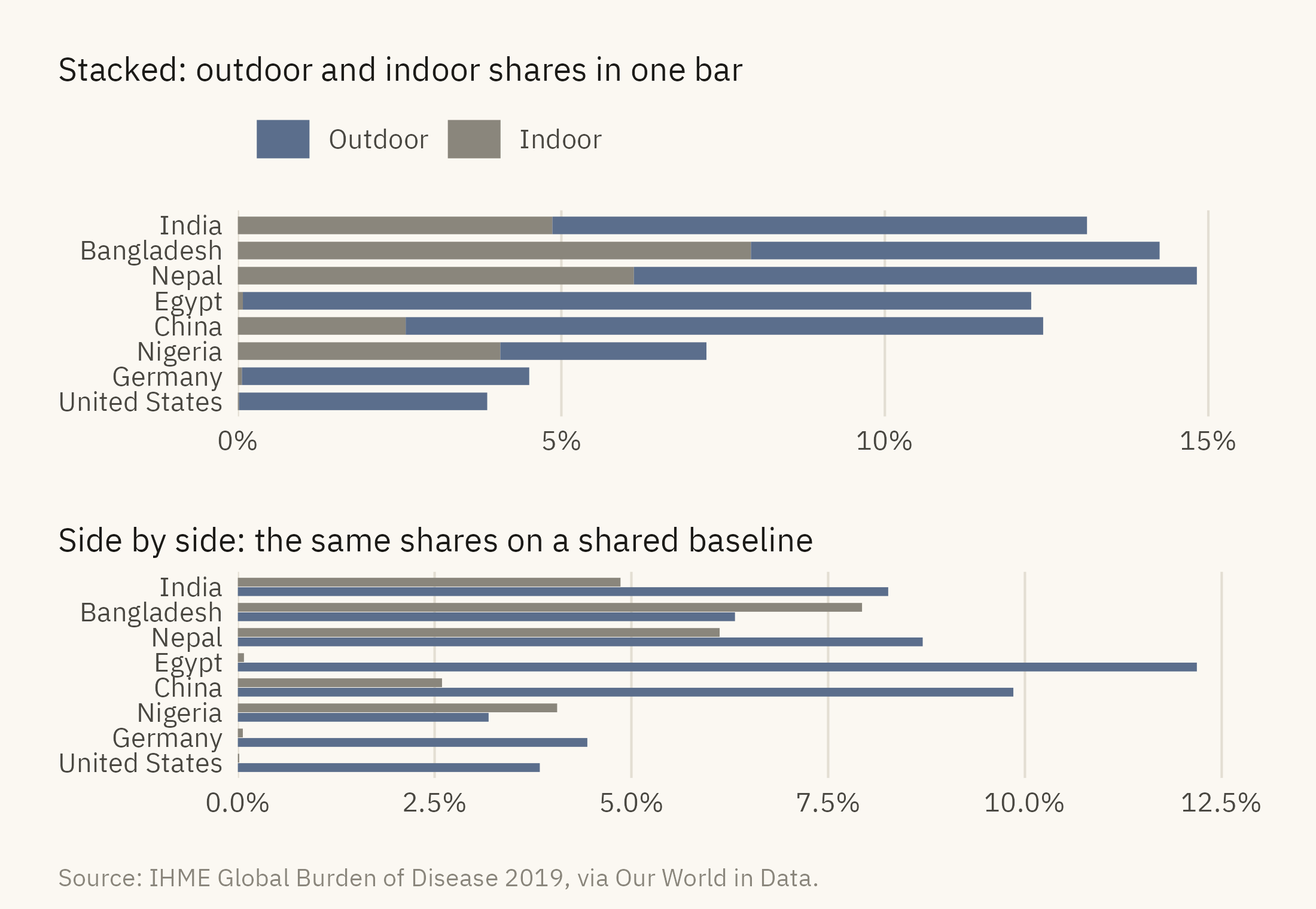
The hierarchy also separates its first and second entries. In a stacked bar, every segment above the first starts at a different height. To compare those segments, a reader has to compare positions on scales that do not line up. Figure 2.4 splits the deaths attributed to air pollution in eight countries into indoor and outdoor sources.
Show the code
eight <-c("India", "Bangladesh", "Nepal", "Egypt", "China", "Nigeria", "Germany", "United States")src <- deaths |>filter(year ==2017, country %in% eight) |>select(country, Indoor = share_indoor, Outdoor = share_outdoor) |>pivot_longer(-country, names_to ="source", values_to ="share") |>mutate(country =factor(country, levels =rev(eight)),source =factor(source, levels =c("Outdoor", "Indoor")))stacked <-ggplot(src, aes(share, country, fill = source)) +geom_col(width =0.7) +scale_fill_manual(values =c(Outdoor =mv_accent(), Indoor = mv_ink$mute)) +scale_x_continuous(labels =label_percent(scale =1), expand =expansion(mult =c(0, 0.05))) +labs(x =NULL, y =NULL, fill =NULL, title ="Stacked: outdoor and indoor shares in one bar") +theme_mv(base_size =10, grid ="x") +theme(plot.title =element_text(size =rel(1), face ="plain"))dodged <-ggplot(src, aes(share, country, fill = source)) +geom_col(width =0.7, position =position_dodge(width =0.75)) +scale_fill_manual(values =c(Outdoor =mv_accent(), Indoor = mv_ink$mute)) +scale_x_continuous(labels =label_percent(scale =1), expand =expansion(mult =c(0, 0.05))) +labs(x =NULL, y =NULL, fill =NULL, title ="Side by side: the same shares on a shared baseline") +theme_mv(base_size =10, grid ="x") +theme(plot.title =element_text(size =rel(1), face ="plain"), legend.position ="none")(stacked / dodged) +plot_annotation(caption =mv_source("IHME Global Burden of Disease 2019, via Our World in Data"),theme =theme(plot.caption =element_text(size =7.5, hjust =0,color = mv_ink$mute, family =mv_font()),plot.background =element_rect(fill = mv_ink$canvas, color =NA)))
Figure 2.4: Share of all deaths attributed to air pollution in 2017 for eight countries, split by source. In the stacked version, the outdoor segments start at different heights and are hard to compare. In the side by side version, the same segments share a baseline and the reader compares lengths. Source: IHME Global Burden of Disease 2019, via Our World in Data.
In the stacked version, India’s bar ends further to the right than China’s, at 13.1 percent against 12.4. A reader takes India’s outdoor share to be the larger. It is the smaller, at 8.3 percent against China’s 9.9. India’s indoor segment is longer, so its outdoor segment starts further from zero. In the side by side version, the outdoor bars share a baseline, China’s is longer than India’s, and Egypt’s outdoor share is the largest of the eight. Stacked bars are suitable when the total is the main point and the parts are secondary. When the parts are the main point, each part needs its own baseline.
Area Against Length
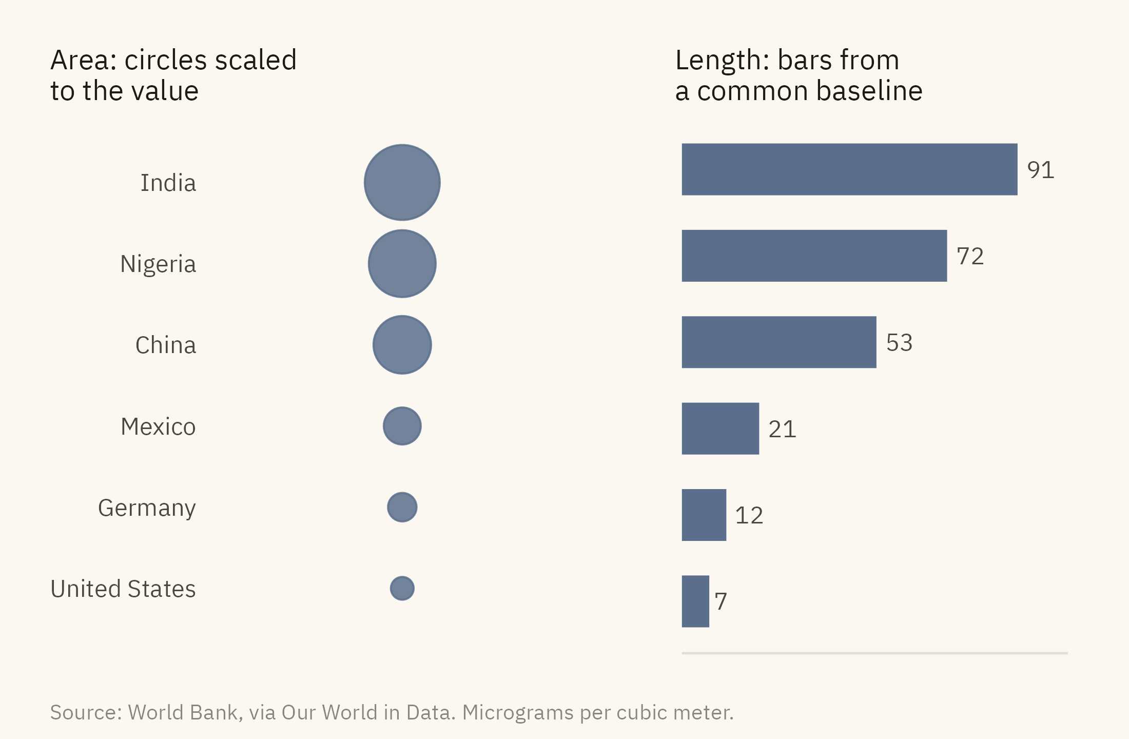
Area is ranked below length for a reason that has been measured since the 1950s. S. S. Stevens showed that perceived area grows more slowly than true area. A circle with twice the area of another looks about 1.6 times as large. Readers therefore underestimate large values, and the differences a chart was drawn to show appear smaller than they are.
Show the code
six <- pm |>filter(year ==2017, country %in%c("India", "Nigeria", "China", "Mexico", "Germany", "United States")) |>mutate(country =fct_reorder(country, pm25))circles <-ggplot(six, aes(x =1, y = country, size = pm25)) +geom_point(color =mv_accent(), alpha =0.85) +scale_size_area(max_size =12, guide ="none") +scale_x_continuous(limits =c(0.5, 1.5)) +scale_y_discrete(expand =expansion(add =0.8)) +labs(x =NULL, y =NULL, title ="Area: circles scaled\nto the value") +theme_mv_blank(base_size =10) +theme(axis.text.y =element_text(size =rel(0.85), color = mv_ink$ink2),plot.title =element_text(size =rel(1), face ="plain"))bars <-ggplot(six, aes(pm25, country)) +geom_col(fill =mv_accent(), width =0.6) +geom_text(aes(label =round(pm25)), hjust =-0.3, size =3, family =mv_font(), color = mv_ink$ink2) +scale_x_continuous(expand =expansion(mult =c(0, 0.15))) +labs(x =NULL, y =NULL, title ="Length: bars from\na common baseline") +theme_mv(base_size =10, grid ="none") +theme(axis.text.x =element_blank(), axis.text.y =element_blank(),plot.title =element_text(size =rel(1), face ="plain"))circles + bars +plot_annotation(caption =mv_source("World Bank, via Our World in Data", "micrograms per cubic meter"),theme =theme(plot.caption =element_text(size =7.5, hjust =0,color = mv_ink$mute, family =mv_font()),plot.background =element_rect(fill = mv_ink$canvas, color =NA)))
Figure 2.5: Mean annual PM2.5 exposure in 2017 for six countries, as circles scaled by area and as bars. India’s exposure is twelve times that of the United States. In the circles, the ratio looks like three or four times. In the bars, it looks like twelve. Source: World Bank, via Our World in Data.
Bubbles are useful for two purposes. They can add a third variable to a scatter plot, and they fit many categories into a small space. The price is accuracy. Use bubbles when the reader only needs to see that one value is larger than another. Use length or position when the reader needs to judge by how much.
2.5 Gestalt: How Marks Become Groups
A reader does not see the marks on a chart as a set of separate objects. The visual system groups them into clusters, paths, regions, and shapes, and the designer decides which grouping the reader will see, often without noticing the decision. The Gestalt psychologists described the rules of grouping a century ago. Five of them account for most of what happens in chart design.
Proximity. Marks that are close together are seen as a group. Faceted charts rely on this. Everything inside one panel is read as belonging together.
Similarity. Marks that share a color or a shape are seen as a group, wherever they are on the page.
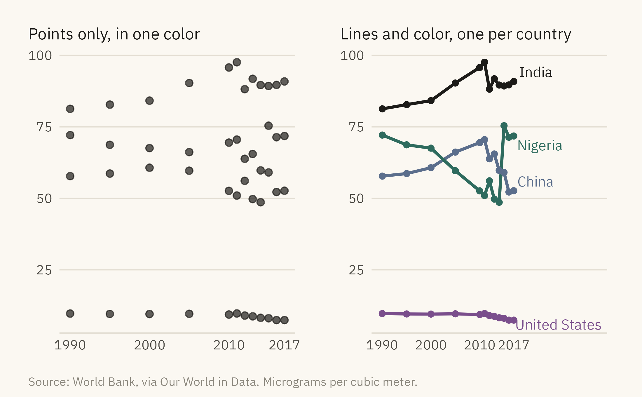
Connection. Marks joined by a line are seen as one object. A line chart of four countries is read as four quantities changing over time. A scatter plot of the same points is read as separate observations.
Enclosure. Marks inside a boundary are seen as a group even when they differ in color or shape. A shaded band or a box produces this effect.
Figure and ground. Some elements are seen as foreground and receive attention. Others are seen as background and do not. Gridlines, backgrounds, and borders belong in the background, and the data belongs in the foreground. Chart junk is the term for a chart in which the two are reversed.
Show the code
four <- pm |>filter(country %in%c("India", "China", "Nigeria", "United States"))ends <- four |>filter(year ==2017)cloud <-ggplot(four, aes(year, pm25)) +geom_point(size =1.8, color = mv_ink$ink, alpha =0.7) +scale_x_continuous(breaks =c(1990, 2000, 2010, 2017)) +labs(x =NULL, y =NULL, title ="Points only, in one color") +theme_mv(base_size =10) +theme(plot.title =element_text(size =rel(1), face ="plain"))paths <-ggplot(four, aes(year, pm25, color = country)) +geom_line(linewidth =0.9) +geom_point(size =1.4) +mv_label_end(ends, aes(label = country, color = country), nudge_x =1) +scale_color_manual(values =c(India = mv_ink$ink, China =mv_accent(),Nigeria ="#2E6B5E", `United States`="#7A4E8C"), guide ="none") +scale_x_continuous(breaks =c(1990, 2000, 2010, 2017), limits =c(1990, 2034)) +labs(x =NULL, y =NULL, title ="Lines and color, one per country") +theme_mv(base_size =10) +theme(plot.title =element_text(size =rel(1), face ="plain"))cloud + paths +plot_annotation(caption =mv_source("World Bank, via Our World in Data", "micrograms per cubic meter"),theme =theme(plot.caption =element_text(size =7.5, hjust =0,color = mv_ink$mute, family =mv_font()),plot.background =element_rect(fill = mv_ink$canvas, color =NA)))
Figure 2.6: PM2.5 exposure for four countries, 1990 to 2017, drawn twice. Left: the points are unconnected and in one color, and a reader sees a cloud. Right: lines connect each country’s points, color separates the countries, and a direct label replaces the legend. Source: World Bank, via Our World in Data.
The right panel of Figure 2.6 also shows a finding that is hard to see in the left panel. India’s exposure rose until 2011 and then fell back to about 90. China’s fell after 2011. The data are the same in both panels. Only the grouping differs.
2.6 Color
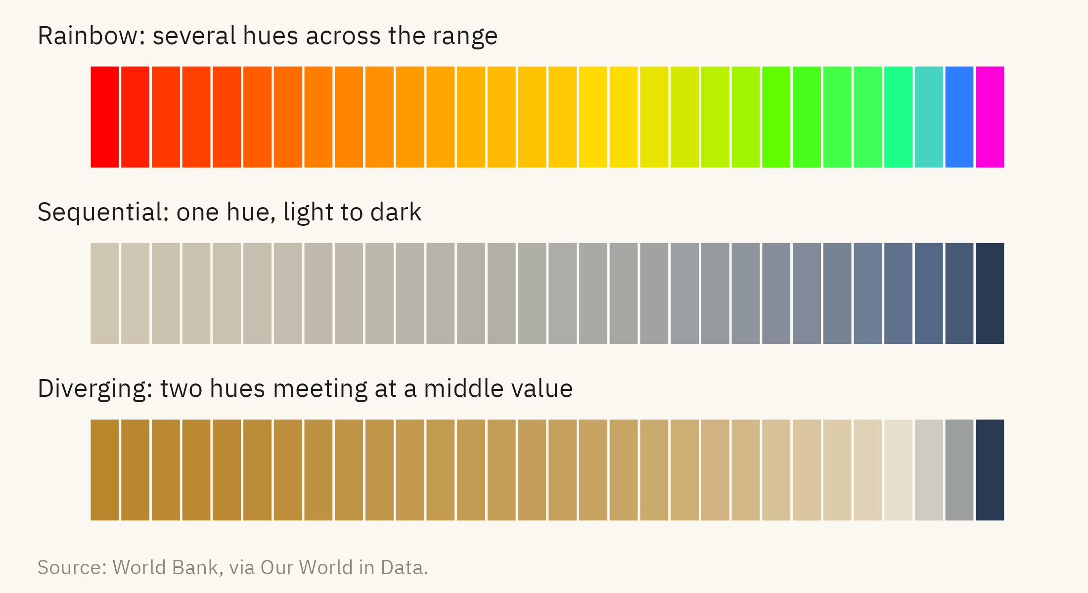
Color is the most common encoding after position and length, and it is often used badly. One reason is that color has more than one dimension. Hue is the name of the color, such as red, blue, or green. Intensity is how light or dark the color is. Hue is suitable for categories, and intensity is suitable for ordered values. A rainbow palette mixes the two. It produces an order that a reader can see but cannot judge accurately, because the step from yellow to green looks larger than the step from blue to violet even when the values are evenly spaced.
Show the code
thirty <- pm |>filter(year ==2017, !is.na(region)) |>arrange(desc(pm25)) |>slice(seq(1, 190, by =6)) |>slice_head(n =30) |>arrange(pm25) |>mutate(rank =row_number())strip <-function(scale, title) {ggplot(thirty, aes(rank, 1, fill = pm25)) +geom_tile(color = mv_ink$canvas, linewidth =0.4) + scale +labs(title = title, x =NULL, y =NULL) +theme_mv_blank(base_size =10) +theme(legend.position ="none", plot.title =element_text(size =rel(0.95), face ="plain"),plot.margin =margin(4, 8, 4, 8))}strip(scale_fill_gradientn(colors =rainbow(7)), "Rainbow: several hues across the range") /strip(scale_fill_gradientn(colors =colorRampPalette(c("#CFC6B2", mv_accent(), "#2A3A52"))(9)),"Sequential: one hue, light to dark") /strip(scale_fill_gradientn(colors =colorRampPalette(c("#B8862B", "#E8E2D4", "#2A3A52"))(9)),"Diverging: two hues meeting at a middle value") +plot_annotation(caption =mv_source("World Bank, via Our World in Data"),theme =theme(plot.caption =element_text(size =7.5, hjust =0,color = mv_ink$mute, family =mv_font()),plot.background =element_rect(fill = mv_ink$canvas, color =NA)))
Figure 2.7: The same thirty countries, sorted by PM2.5 exposure in 2017 from low on the left to high on the right, shaded three ways. The rainbow adds boundaries that are not in the data. The single-hue ramp shows a smooth ordering. The diverging ramp does not fit here. Its light middle falls at 55 micrograms, between the 27th and 28th tiles, because the data has no meaningful center. Source: World Bank, via Our World in Data.
Three families of color scale cover nearly every case. A qualitative scale uses distinct hues for unordered categories. A sequential scale uses one hue from light to dark for values that run from low to high. A diverging scale uses two hues that meet at a neutral middle. It is suitable for values with a meaningful zero or center, such as change from a baseline or a vote margin. The data decide which family fits.
About one man in twelve and one woman in two hundred cannot reliably tell red from green. A chart whose two main colors are red and green cannot be read by that share of its audience. Two remedies are available, and both are easy to apply. The first is to choose palettes designed for color-vision deficiency, such as viridis or the ColorBrewer colorblind-safe sets. The second is to show any category in a second channel as well, such as a shape, a label, or a line pattern. This is called double encoding, and it keeps a chart readable in color, in grayscale, and on a photocopy.
2.7 The Baseline
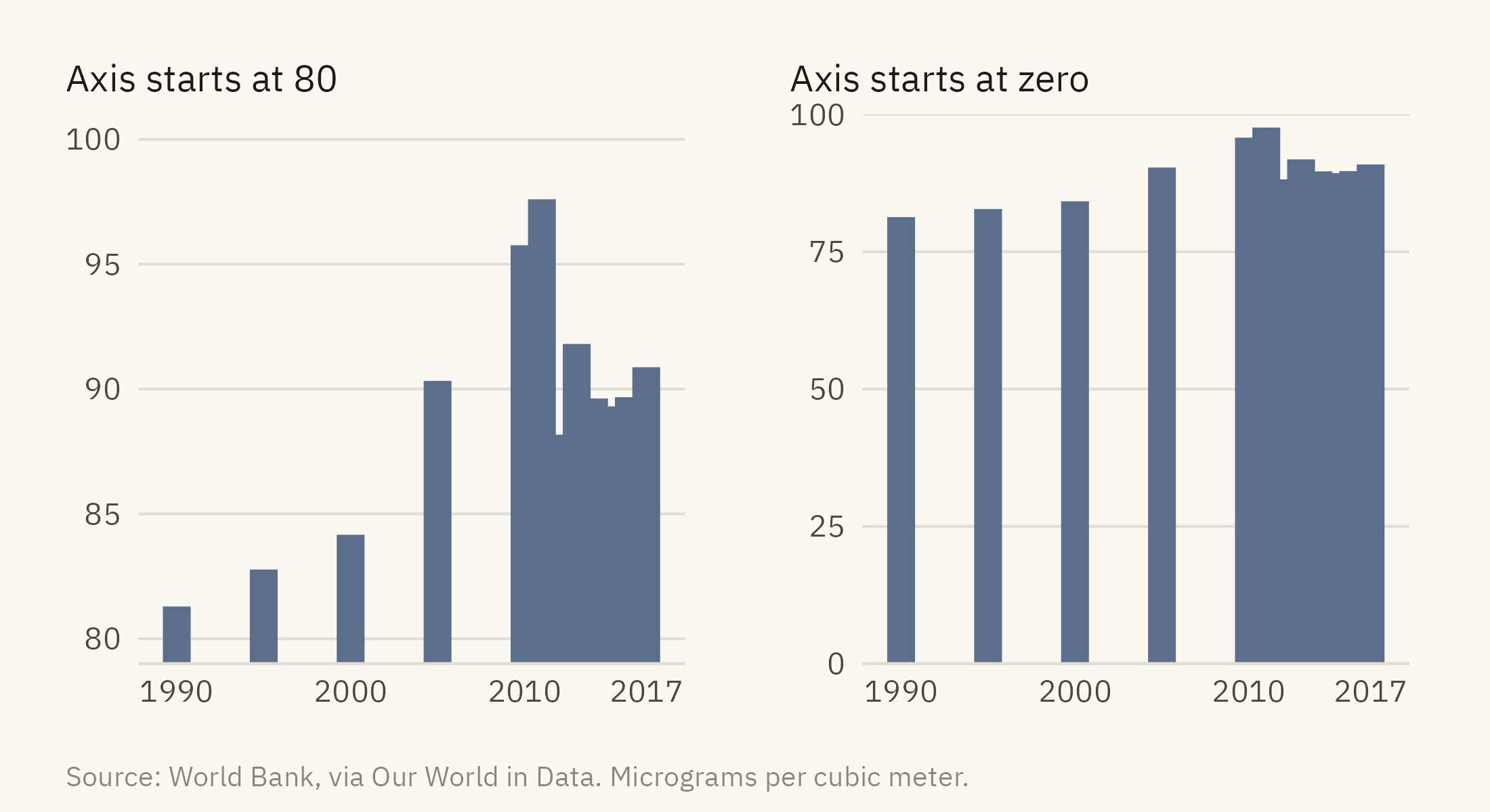
One perceptual rule needs its own section because it is broken so often. A bar encodes a value as length measured from a baseline. If the baseline is not zero, the length no longer corresponds to the value, and the comparison a reader makes between bars is wrong by an amount the chart does not reveal. Figure 2.8 shows India’s PM2.5 exposure since 1990, drawn twice.
Show the code
india <- pm |>filter(country =="India")trunc <-ggplot(india, aes(year, pm25)) +geom_col(fill =mv_accent(), width =1.6) +coord_cartesian(ylim =c(80, 100)) +scale_y_continuous(breaks =seq(80, 100, 5)) +scale_x_continuous(breaks =c(1990, 2000, 2010, 2017)) +labs(x =NULL, y =NULL, title ="Axis starts at 80") +theme_mv(base_size =10) +theme(plot.title =element_text(size =rel(1), face ="plain"))full <-ggplot(india, aes(year, pm25)) +geom_col(fill =mv_accent(), width =1.6) +scale_y_continuous(limits =c(0, 100), expand =expansion(0)) +scale_x_continuous(breaks =c(1990, 2000, 2010, 2017)) +labs(x =NULL, y =NULL, title ="Axis starts at zero") +theme_mv(base_size =10) +theme(plot.title =element_text(size =rel(1), face ="plain"))trunc + full +plot_annotation(caption =mv_source("World Bank, via Our World in Data", "micrograms per cubic meter"),theme =theme(plot.caption =element_text(size =7.5, hjust =0,color = mv_ink$mute, family =mv_font()),plot.background =element_rect(fill = mv_ink$canvas, color =NA)))
Figure 2.8: PM2.5 exposure in India, 1990 to 2017, drawn twice. Left: the vertical axis starts at 80 and the rise from 1990 to 2017 looks about eightfold. Right: the axis starts at zero and the rise is 12 percent. Both panels use the same numbers. Only the right one lets the reader judge the size of the change. Source: World Bank, via Our World in Data.
Tufte called the ratio of the effect as drawn to the effect in the data the lie factor. For a bar chart, it is the apparent change divided by the true change. On the left of Figure 2.8, the 2017 bar is 8.4 times the height of the 1990 bar, an apparent rise of 740 percent. The true rise is 12 percent. The lie factor is about 60. The rule that follows is short. Bars start at zero. Lines and points may start elsewhere, because they encode position rather than length. A chart of a value that never approaches zero can start its axis above zero, but the axis should say so, and the reader should be able to see the reason.
2.8 Data Ink and Other Ink
Tufte’s second lasting idea is the data-ink ratio. Ink spent on the data shows the message. Ink spent on anything else competes with it. Heavy gridlines, borders, shaded backgrounds, drop shadows, and an unneeded legend are all ink of the second kind. The strong form of the argument, that all decoration is harmful, has not been supported in experiments. Some embellishment helps a reader remember a chart. The weak form has been supported. Every mark that is not data should be kept only if removing it would make the chart harder to read.
Show the code
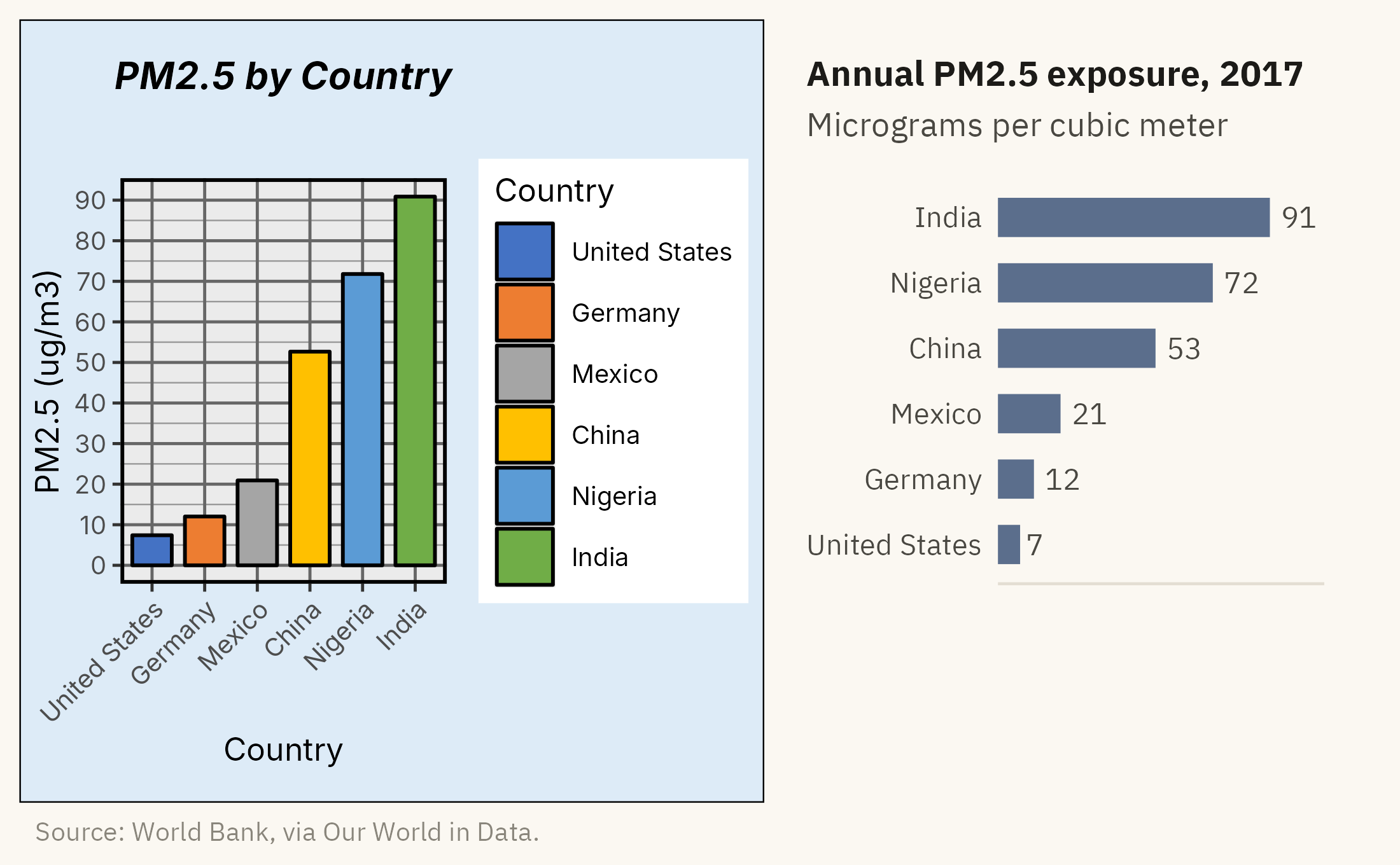
junk <-ggplot(six, aes(country, pm25, fill = country)) +geom_col(color ="black", width =0.75) +scale_fill_manual(values =c("#4472C4", "#ED7D31", "#A5A5A5", "#FFC000", "#5B9BD5", "#70AD47")) +scale_y_continuous(breaks =seq(0, 100, 10), minor_breaks =seq(0, 100, 5)) +labs(x ="Country", y ="PM2.5 (ug/m3)", fill ="Country", title ="PM2.5 by Country") +theme_gray(base_size =9) +theme(panel.grid.major =element_line(color ="grey40"), panel.grid.minor =element_line(color ="grey60"),panel.border =element_rect(fill =NA, color ="black", linewidth =1),plot.background =element_rect(fill ="#DDEBF7", color ="black"),axis.text.x =element_text(angle =45, hjust =1),plot.title =element_text(face ="bold.italic", hjust =0.5))clean <-ggplot(six, aes(pm25, country)) +geom_col(fill =mv_accent(), width =0.6) +geom_text(aes(label =round(pm25)), hjust =-0.3, size =3, family =mv_font(), color = mv_ink$ink2) +scale_x_continuous(expand =expansion(mult =c(0, 0.2))) +labs(x =NULL, y =NULL, title ="Annual PM2.5 exposure, 2017",subtitle ="Micrograms per cubic meter") +theme_mv(base_size =10, grid ="none") +theme(axis.text.x =element_blank(), plot.title =element_text(size =rel(1)))junk + clean +plot_annotation(caption =mv_source("World Bank, via Our World in Data"),theme =theme(plot.caption =element_text(size =7.5, hjust =0,color = mv_ink$mute, family =mv_font()),plot.background =element_rect(fill = mv_ink$canvas, color =NA)))
Figure 2.9: The six-country exposure chart drawn with spreadsheet defaults and again with the non-data ink removed. The data is identical in both. Source: World Bank, via Our World in Data.
The right panel of Figure 2.9 contains the same information as the left. The legend was removed because the labels already name the countries. The gridlines were removed because the values are printed. The colors were removed because the bars show one variable, and six hues suggested six categories. What remains is the data and the words needed to read it.
2.9 The Final Chart
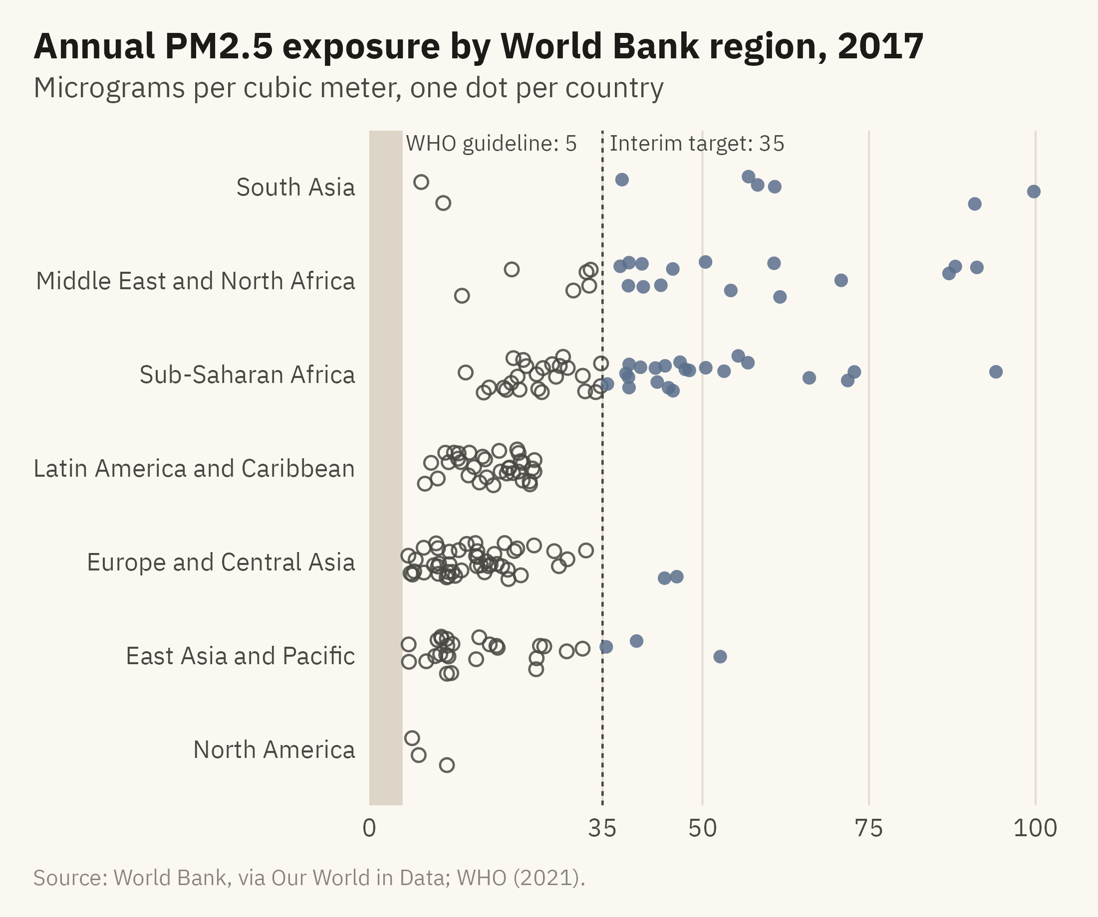
Each demonstration in this chapter addressed one part of the case, and Figure 2.10 combines them. The values are placed along a common scale, which is the encoding readers judge most accurately. A shaded band marks the guideline. One accent color and a filled dot mark the countries above the interim target. The filled dot keeps that group visible in grayscale. Direct labels replace a legend, and the axis starts at zero.
Show the code
now <- pm |>filter(year ==2017, !is.na(region)) |>mutate(region =str_replace(region, " & ", " and "),region =fct_reorder(region, pm25, .fun = median),over35 = pm25 >35)set.seed(7)ggplot(now, aes(pm25, region)) +annotate("rect", xmin =0, xmax =5, ymin =-Inf, ymax =Inf, fill ="#D9D2C2", alpha =0.9) +annotate("text", x =5.5, y =Inf, label ="WHO guideline: 5", hjust =0, vjust =1.3,size =2.8, family =mv_font(), color = mv_ink$ink2) +geom_vline(xintercept =35, linetype ="22", color = mv_ink$ink2, linewidth =0.4) +annotate("text", x =36, y =Inf, label ="Interim target: 35", hjust =0, vjust =1.3,size =2.8, family =mv_font(), color = mv_ink$ink2) +geom_jitter(aes(color = over35, shape = over35), height =0.2, width =0, size =1.9,alpha =0.85, stroke =0.6) +scale_color_manual(values =c(`FALSE`= mv_ink$ink2, `TRUE`=mv_accent()), guide ="none") +scale_shape_manual(values =c(`FALSE`=1, `TRUE`=16), guide ="none") +scale_x_continuous(expand =expansion(mult =c(0, 0.03)), breaks =c(0, 35, 50, 75, 100)) +labs(title ="Annual PM2.5 exposure by World Bank region, 2017",subtitle ="Micrograms per cubic meter, one dot per country",x =NULL, y =NULL,caption =mv_source("World Bank, via Our World in Data; WHO (2021)")) +theme_mv(grid ="x")
Figure 2.10: Population-weighted annual PM2.5 exposure in 2017, one dot per country, grouped by World Bank region. The shaded band is the WHO guideline of 5 micrograms per cubic meter. No country meets it. The filled dots in the accent color, to the right of the dashed line, are the 48 countries above 35, the WHO’s loosest interim target. Source: World Bank, via Our World in Data; WHO Global Air Quality Guidelines (2021).
The chart answers the question raised at the start of the case. A reader can see, without arithmetic, how far each country is from the guideline and which countries are above the interim target. The shaded band on the left contains no dots, because no country meets the guideline.
ImportantEthics Moment: Whom Are You Designing For?
Perception varies across the people who will read your chart. Some cannot separate red from green. Many read on a phone in poor light. Some use a screen reader and will not see the chart at all. Every choice described in this chapter, the encoding, the palette, and how much to label, determines which of these readers the chart includes. There is no neutral default. A chart that can only be read by someone with good color vision, a large screen, and time to study it has an audience that the designer chose, whether or not the designer meant to choose it.
TipTry It Online
The Perception Lab at viz.marginoferrormedia.com/apps runs the Cleveland and McGill experiment on you. It shows pairs of values encoded as positions, lengths, angles, areas, and shades, asks for the ratio, and records your error. After twenty rounds it draws your own hierarchy. A second tab times how fast you find a target by color, size, shape, and orientation, and shows what happens when the target is defined by two features at once.
WarningAI Reality Check: Default Encodings
Ask a language model for a chart of a category breakdown and the first draft is often a pie chart, sometimes with a 3D tilt. Ask for a heatmap and the palette is often a rainbow. Ask for two related quantities and the draft is often a dual-axis chart. Ask for anything with two groups and the colors are often red and green. These defaults come from the training data, which contains a great deal of spreadsheet output designed for visual interest rather than accuracy.
The numbers in a generated chart are usually correct. The encoding is where the problems appear, and the tool does not say which encoding it chose or why. Read a generated chart the way you would read a draft from an analyst who has not yet learned the hierarchy, and check it against the rules in this chapter. Position before length. Length before angle or area. One hue for one variable. Bars from zero. No ink that does not help the reader.
2.10 Putting It All Together
Readers judge some encodings accurately and others poorly, and the ranking has been measured. Position and length are judged accurately. Angle, area, and shade are not. A chart whose main comparison uses an encoding near the top of the hierarchy will be read correctly by more people with less effort. The Gestalt rules determine what readers see as a group, and a designer who does not choose the grouping will get one anyway. Hue is suitable for categories, intensity for ordered values, and a palette that mixes the two misleads. Bars start at zero. Non-data ink is kept only when it helps the reader. The air pollution chart at the end of the chapter applies these rules in order.
2.11 Looking Ahead
Chapter 3 reverses the point of view. Instead of making a chart, you will read charts that other people made. Several of them come from recent news coverage of immigration, and you will examine them with the rules from this chapter. That skill has become more useful now that software draws the first draft. Part II then applies the rules to the choice of chart, one question at a time: comparison, distribution, relationship, change, and place.
2.12 Further Reading and References
Bateman, S., Mandryk, R. L., Gutwin, C., Genest, A., McDine, D., and Brooks, C. (2010). Useful junk? The effects of visual embellishment on comprehension and memorability of charts. Proceedings of CHI 2010, 2573–2582. The experiment that limits the strong form of the data-ink argument.
Cleveland, W. S., and McGill, R. (1984). Graphical perception: Theory, experimentation, and application to the development of graphical methods. Journal of the American Statistical Association, 79(387), 531–554. The original hierarchy.
Crameri, F., Shephard, G. E., and Heron, P. J. (2020). The misuse of colour in science communication. Nature Communications, 11, 5444. The case against rainbow palettes, with examples from published science.
Dalal, S. R., Fowlkes, E. B., and Hoadley, B. (1989). Risk analysis of the space shuttle: Pre-Challenger prediction of failure. Journal of the American Statistical Association, 84(408), 945–957. The O-ring data and the statistical analysis that could have been done before the launch.
Heer, J., and Bostock, M. (2010). Crowdsourcing graphical perception: Using Mechanical Turk to assess visualization design. Proceedings of CHI 2010, 203–212. The large-scale replication of Cleveland and McGill.
Robison, W., Boisjoly, R., Hoeker, D., and Young, S. (2002). Representation and misrepresentation: Tufte and the Morton Thiokol engineers on the Challenger. Science and Engineering Ethics, 8(1), 59–81. The engineers’ reply to Tufte, with Boisjoly as a co-author.
Treisman, A., and Gelade, G. (1980). A feature-integration theory of attention. Cognitive Psychology, 12(1), 97–136. The two-stage model of visual processing.
Tufte, E. R. (1997). Visual Explanations. Graphics Press. The Challenger chapter.
Tufte, E. R. (2001). The Visual Display of Quantitative Information, 2nd edition. Graphics Press. The lie factor and the data-ink ratio.
World Health Organization (2021). WHO Global Air Quality Guidelines. The 5 microgram guideline and the interim targets used in the chapter.
2.13 Key Terms
Preattentive processing. The fast, parallel, automatic stage of vision that detects color, position, size, and orientation before attention is directed.
Cleveland and McGill hierarchy. The ranking of visual encodings by how accurately readers compare quantities, from position (best) to volume (worst).
Gestalt principles. Proximity, similarity, connection, enclosure, and figure-and-ground. The rules by which the visual system groups marks into objects.
Hue and intensity. The two dimensions of color that matter for charts. Hue names the color and suits categories, and intensity is lightness and suits ordered values.
Qualitative, sequential, diverging. The three families of color scale, for categories, for ordered values, and for values with a meaningful center.
Double encoding. Showing a category in two channels, such as color and shape, so the chart stays readable with color-vision deficiency and in grayscale.
Lie factor. The ratio of the size of an effect as drawn to the size of the effect in the data. It should be close to one.
Data-ink ratio. The share of a chart’s ink that shows data. Non-data ink stays only when it helps the reader.
2.14 Exercises
Check Your Understanding
Rank these four encodings from most to least accurately decoded: the angle of a pie slice, the length of a bar, the shade of a map region, the position of a dot on a shared axis.
Figure 2.4 shows the same values stacked and side by side. Which Gestalt principle makes the stacked version read as “one bar per country,” and why does that reading make the parts harder to compare?
Explain why a line chart of four countries is read differently from a scatter plot of the same points. Name the principle.
A colleague argues that the truncated axis in Figure 2.8 is fine because “the reader can see the axis labels.” Reply in two sentences using the idea of the lie factor.
For each dataset, say whether a qualitative, sequential, or diverging palette fits. County unemployment rates. The party that won each state. Change in a city’s population since 2010.
Apply It
Using ch02-pm25-exposure.csv, draw the 2017 exposure for the ten most populous countries as a pie chart and as a dot plot. Write down, before looking at the numbers, which country is third from the pie. Then check.
Redraw Figure 2.10 with the countries colored by income group rather than by the 35 threshold. Does the chart still have one accent color? If not, decide which version directs the reader’s attention better and why.
Take any chart from a recent news article and list every mark that is not data. For each, say whether removing it would hurt the chart.
Draw the four-country line chart from Figure 2.6 in grayscale and with a legend instead of direct labels. Describe what the reader loses.
Think Deeper
The hierarchy ranks position above length, yet bar charts are far more common than dot plots in business reports. Offer two reasons that are not about accuracy, and say whether either is a good reason.
The Ethics Moment says there is no neutral default. Choose one default in your own charting tool, such as its color palette or its gridlines, and say which readers it serves well and which it serves badly.
Tufte’s redrawing of the Challenger data has been criticized for putting the engineers in a bad light. Read the Robison and colleagues reply and write a paragraph on what the chart can and cannot be blamed for.