Most of the charts a reader sees were made by someone else. They appear in news stories, on slides in meetings, and in posts shared online. The first two chapters were about making charts. This chapter is about reading them. Software now draws the first draft of most charts. Whether to accept a chart is still a judgment made by the reader, and this chapter gives a procedure for making that judgment.
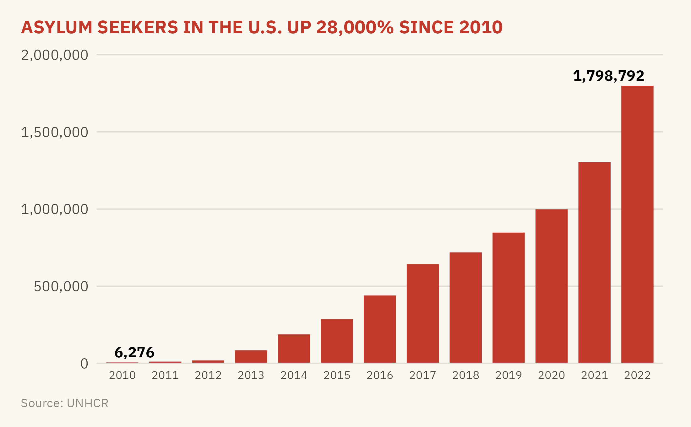
The case for this chapter is a bar chart that was widely shared during the debate over immigration enforcement. It showed the number of asylum seekers in the United States each year from 2010 to 2022. The headline above the chart said the number had risen by more than 28,000 percent. Every number on the chart was correct. Figure 3.1 is that chart, redrawn from the UNHCR data it cited.
Show the code
ggplot(us_year, aes(factor(year), asylum)) +geom_col(fill ="#C0392B", width =0.75) +geom_text(data =filter(us_year, year %in%c(2010, 2022)),aes(label =label_comma()(asylum), hjust =c(0.2, 0.9)), vjust =-0.5, size =3, family =mv_font(), fontface ="bold") +scale_y_continuous(labels =label_comma(), expand =expansion(mult =c(0, 0.15))) +labs(title ="ASYLUM SEEKERS IN THE U.S. UP 28,000% SINCE 2010",x =NULL, y =NULL, caption ="Source: UNHCR") +theme_mv(base_size =10) +theme(plot.title =element_text(color ="#C0392B", size =rel(1.05)),axis.text.x =element_text(size =rel(0.8)))
Figure 3.1: A chart of the kind that circulated during the immigration enforcement debate, redrawn from the UNHCR data it cited. The numbers are accurate. The unit is not stated, and the series counts pending claims rather than arrivals. Source: UNHCR Refugee Population Statistics Database.
The chart is not false. Every bar is accurate. The problems are in what the chart leaves out and in the conclusion the headline draws from it. This chapter examines the chart with seven questions, asked in order. The seven questions form the reading protocol this chapter teaches. They apply to any chart, including the ones you make yourself.
3.2 Question 1: What Is Being Counted?
Every chart shows a count or a measure of something, and the title often does not say what the unit is. The first step is to find the unit and ask whether a reader is likely to misread it. The most common confusion is between a stock and a flow. A flow is the number of events during a period, such as arrivals in a year, sales in a quarter, or deaths in a month. A stock is the number of things that exist at one moment, such as people in the country on December 31, inventory in a warehouse, or cases pending on a court docket.
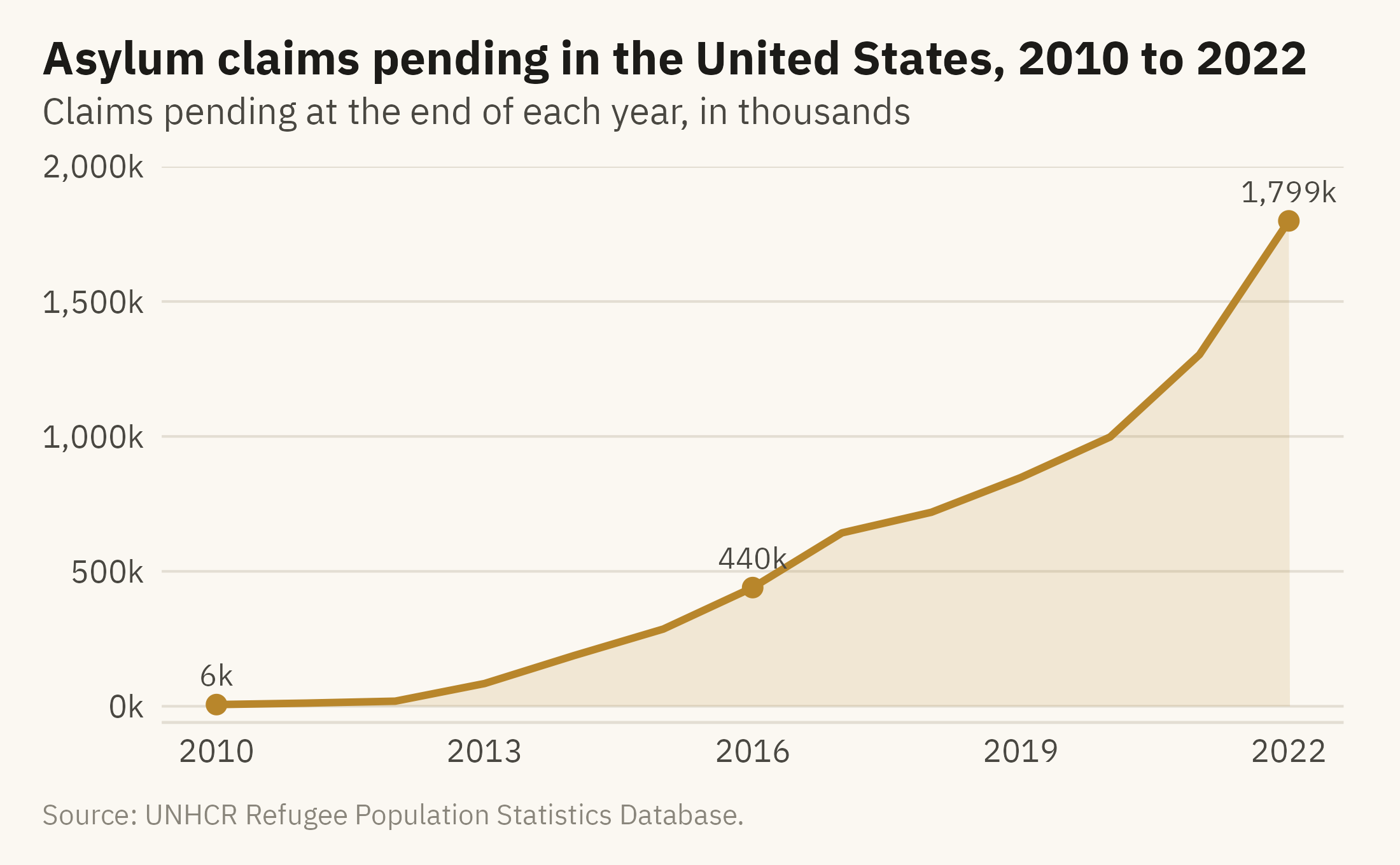
UNHCR’s “asylum-seekers” figure is a stock. Under the UNHCR methodology (2023), it counts people whose claims were still pending at the end of the year. A claim filed in 2016 and still undecided in 2022 is counted in each of those seven years. The bars in the viral chart therefore show the size of the backlog at the end of each year, not the number of people who sought asylum during the year. The two quantities have different causes. The number of new claims depends on arrivals. The size of the backlog depends on new claims and on the rate at which claims are decided.
Show the code
ggplot(us_year, aes(year, asylum)) +geom_area(fill =mv_accent(), alpha =0.15) +geom_line(color =mv_accent(), linewidth =1) +geom_point(data =filter(us_year, year %in%c(2010, 2016, 2022)), color =mv_accent(), size =2.2) +geom_text(data =filter(us_year, year %in%c(2010, 2016, 2022)),aes(label =label_comma(scale =1e-3, suffix ="k", accuracy =1)(asylum)),vjust =-0.9, size =3, family =mv_font(), color = mv_ink$ink2) +scale_x_continuous(breaks =seq(2010, 2022, 3)) +scale_y_continuous(labels =label_comma(scale =1e-3, suffix ="k"), limits =c(0, 2e6),expand =expansion(mult =c(0.03, 0))) +labs(title ="Asylum claims pending in the United States, 2010 to 2022",subtitle ="Claims pending at the end of each year, in thousands",x =NULL, y =NULL, caption =mv_source("UNHCR Refugee Population Statistics Database")) +theme_mv()
Figure 3.2: Asylum claims pending in the United States at the end of each year, 2010 to 2022. The series is a stock, not a count of arrivals. A backlog grows when claims are filed faster than they are decided, so the series depends on the speed of decisions as well as on arrivals. Source: UNHCR Refugee Population Statistics Database.
The 28,000 percent figure is correct for the backlog. What the first question changes is the conclusion. A reader who takes the bars as arrivals might write “asylum seekers flooded in.” A reader who knows the unit would write “pending asylum claims grew.” The second statement concerns the processing of claims as well as arrivals, which is a different policy question.
3.3 Question 2: Where Does the Axis Start?
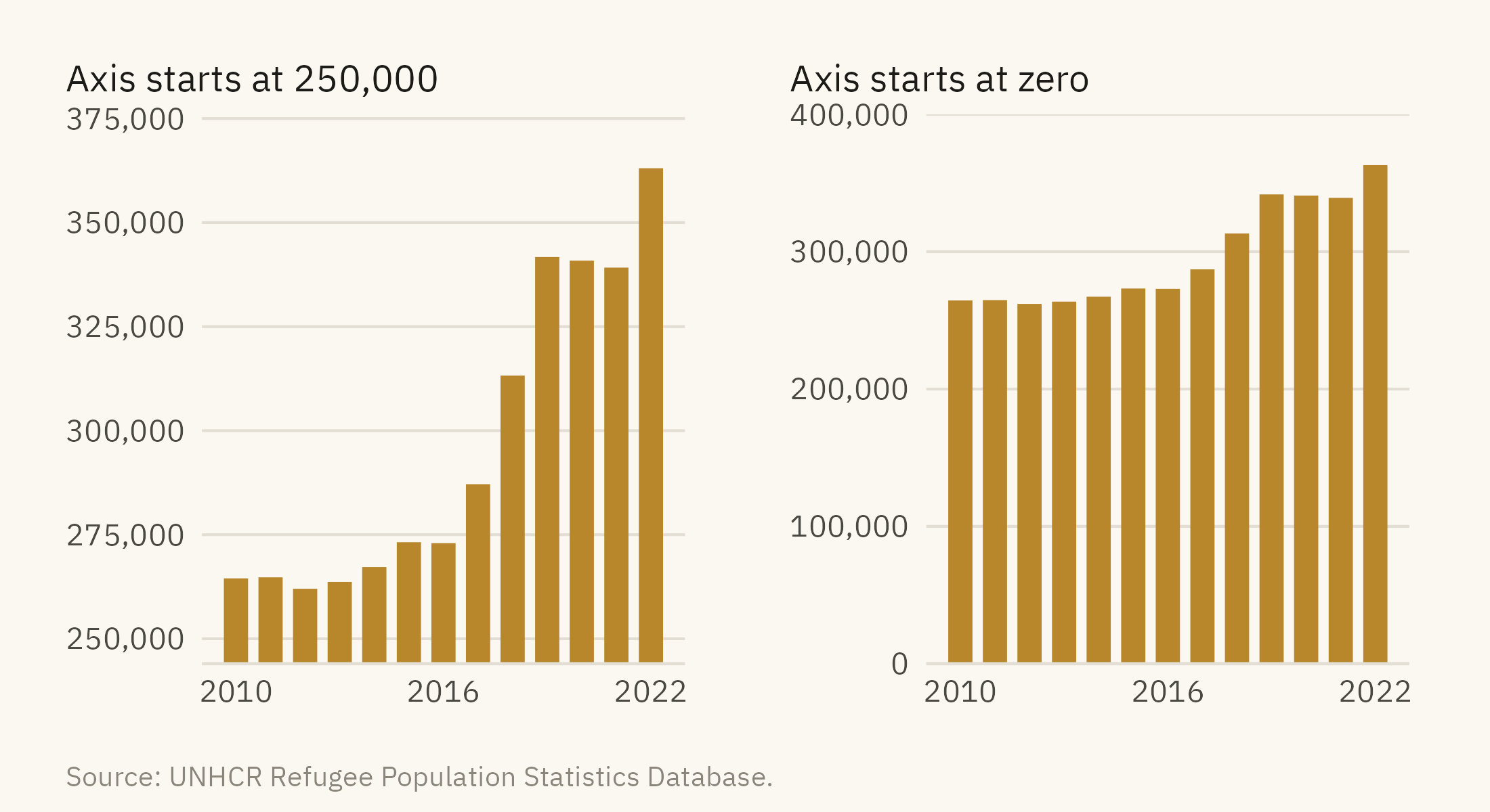
Chapter 2 gave the rule that bars start at zero. The viral chart follows that rule. Many charts do not. Figure 3.3 shows the number of refugees the United States hosted over the same period, drawn two ways. Refugees are a separate category from asylum seekers in the UNHCR data. They were granted protection before they arrived.
Figure 3.3: Refugees hosted by the United States, 2010 to 2022. Left, the axis starts at 250,000, and the bars appear to rise about eightfold. Right, the axis starts at zero, and the rise is 37 percent. Source: UNHCR Refugee Population Statistics Database.
To apply this check, find the lowest value on the vertical axis. If it is not zero and the marks are bars, the bar lengths do not correspond to the values. If the marks are lines or points, a non-zero start can be acceptable. The axis labels should then make the starting value visible.
3.4 Question 3: What Is the Time Window?
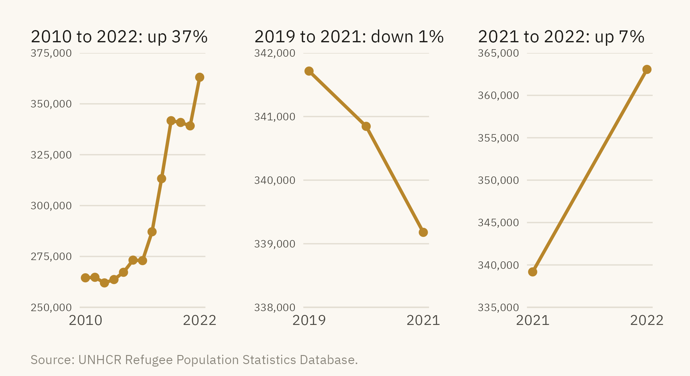
Every time series has a start date and an end date, and the author chose them. A different start date can change the direction of the trend. Figure 3.4 shows the refugee series over three windows. Each window is accurate, and each supports a different summary.
Show the code
win <-function(from, to, title, lo, hi, step) { d <-filter(us_year, year >= from, year <= to)ggplot(d, aes(year, refugees)) +geom_line(color =mv_accent(), linewidth =0.9) +geom_point(color =mv_accent(), size =1.8) +scale_x_continuous(breaks =c(from, to)) +scale_y_continuous(labels =label_comma(), limits =c(lo, hi), breaks =seq(lo, hi, step),expand =expansion(0)) +labs(x =NULL, y =NULL, title = title) +theme_mv(base_size =10) + plain_title +theme(axis.text.y =element_text(size =rel(0.75)))}win(2010, 2022, "2010 to 2022: up 37%", 250000, 375000, 25000) +win(2019, 2021, "2019 to 2021: down 1%", 338000, 342000, 1000) +win(2021, 2022, "2021 to 2022: up 7%", 335000, 365000, 5000) +plot_annotation(caption =mv_source("UNHCR Refugee Population Statistics Database"), theme = cap_theme)
Figure 3.4: Refugees hosted by the United States, drawn over three time windows. From 2010 to 2022, the series rises 37 percent. From 2019 to 2021, it falls 1 percent. From 2021 to 2022, it rises 7 percent. Each panel has its own vertical axis, and none starts at zero. The middle axis spans 4,000 people, so a fall of 2,500 fills the panel. The direction and the apparent size of the trend both depend on choices the author made. Source: UNHCR Refugee Population Statistics Database.
The longest window the data allows is usually the most informative, because any shorter window can be seen within it. When a chart shows a short window, a reader should ask what the full series shows and why the series starts where it does. The viral chart starts in 2010 because the UNHCR open data series starts in 2010. A chart that started in 2016, when the backlog was already 440,000, would have had no such reason.
3.5 Question 4: What Is the Denominator?
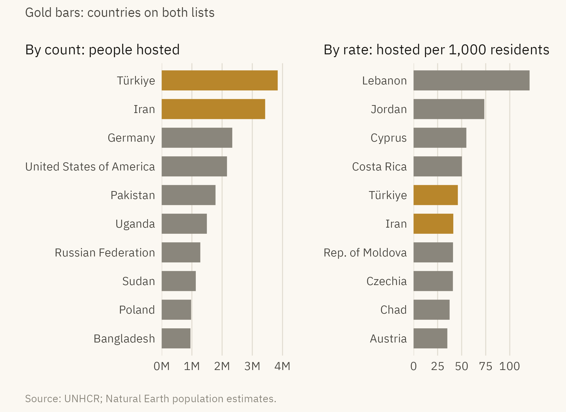
A count describes the size of a group. A rate, which divides the count by a population, describes the size of the group relative to that population. In 2022, the United States hosted more refugees and asylum seekers than any country except Türkiye, Iran, and Germany. Its population was about 330 million. Figure 3.5 shows the ten largest hosts in 2022 by count and by the number hosted per 1,000 residents.
Show the code
top_n <- hosts |>slice_max(hosted, n =10) |>mutate(asylum =fct_reorder(str_replace(asylum, " \\(.*\\)", ""), hosted))top_r <- hosts |>filter(pop_est >1e6) |>slice_max(per_1000, n =10) |>mutate(asylum =fct_reorder(str_replace(asylum, " \\(.*\\)", ""), per_1000))both <-intersect(as.character(top_n$asylum), as.character(top_r$asylum))p1 <-ggplot(top_n, aes(hosted, asylum, fill = asylum %in% both)) +geom_col(width =0.7) +scale_fill_manual(values =c(`FALSE`= mv_ink$mute, `TRUE`=mv_accent()), guide ="none") +scale_x_continuous(labels =label_comma(scale =1e-6, suffix ="M"), expand =expansion(mult =c(0, 0.05))) +labs(x =NULL, y =NULL, title ="By count: people hosted") +theme_mv(base_size =10, grid ="x") + plain_titlep2 <-ggplot(top_r, aes(per_1000, asylum, fill = asylum %in% both)) +geom_col(width =0.7) +scale_fill_manual(values =c(`FALSE`= mv_ink$mute, `TRUE`=mv_accent()), guide ="none") +scale_x_continuous(breaks =seq(0, 100, 25), expand =expansion(mult =c(0, 0.05))) +labs(x =NULL, y =NULL, title ="By rate: hosted per 1,000 residents") +theme_mv(base_size =10, grid ="x") + plain_titlep1 + p2 +plot_annotation(subtitle ="Gold bars: countries on both lists",caption =mv_source("UNHCR; Natural Earth population estimates"),theme = cap_theme +theme(plot.subtitle =element_text(size =9, color = mv_ink$ink2, family =mv_font())))
Figure 3.5: Refugees and asylum seekers hosted in 2022. Left, the ten countries hosting the largest numbers. Right, the ten with the most hosted per 1,000 residents, among countries with over one million people. Only Türkiye and Iran appear on both lists. Source: UNHCR; population from Natural Earth estimates.
The United States is fourth by count. It does not appear on the rate list, since it hosted 6.6 per thousand residents. Lebanon hosted 121 per thousand, or about one resident in eight. The two panels answer different questions. A reader should identify which question the author answered and which the author left out.
3.6 Question 5: Does the Encoding Fit the Question?
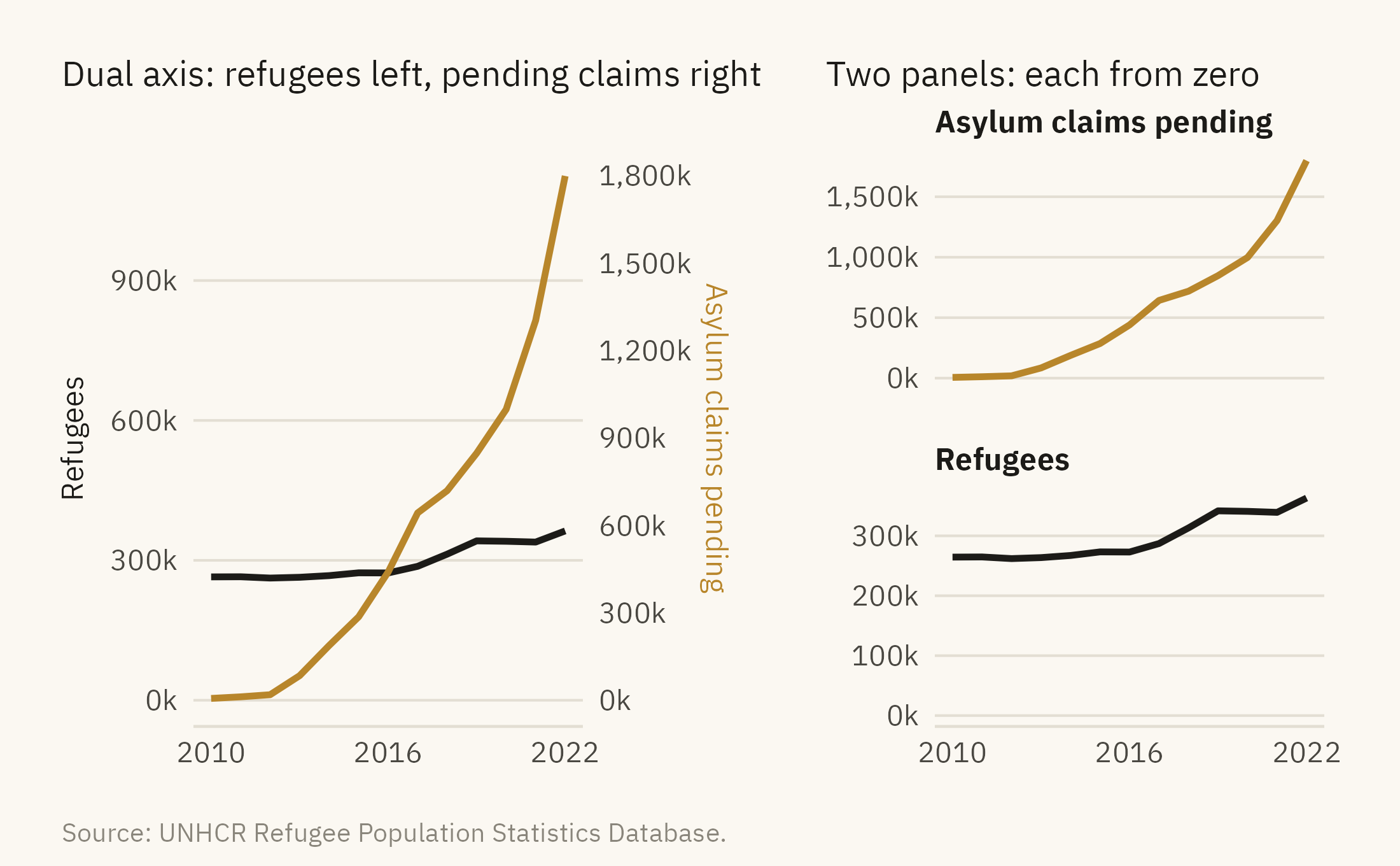
Chapter 2 ranked encodings by how accurately readers judge them. The fifth question asks whether the encoding allows the comparison that the title or the highlight asks the reader to make. Two encodings are common sources of error. The first is the dual axis, which places two series on two vertical scales that share one horizontal axis. Figure 3.6 shows refugees and pending asylum claims on a dual axis and again as two panels.
Figure 3.6: Refugees and pending asylum claims in the United States on a dual-axis chart (left) and as two panels with their own scales (right). On the dual axis, the lines cross in 2016. The crossing exists only because of how the two scales were chosen. Source: UNHCR Refugee Population Statistics Database.
The crossing in the left panel depends on the ratio between the two scales, which the author chose. A different ratio moves the crossing to a different year or removes it. The two panels on the right show each series from zero and do not imply a relationship between them.
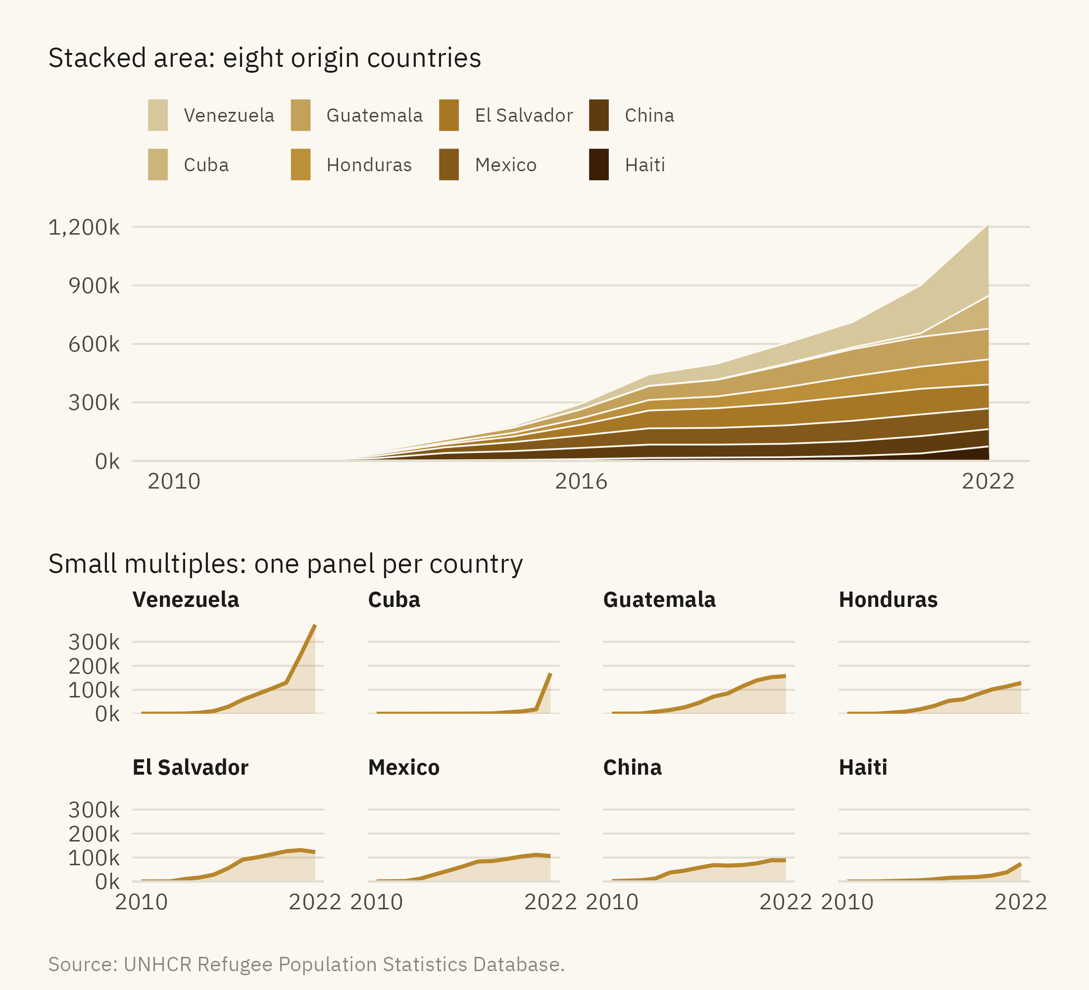
The second pattern is the stacked area chart of many categories. Figure 3.7 shows the origin countries of asylum claims pending in the United States as a stacked area and as small multiples.
Figure 3.7: Pending asylum claims in the United States by country of origin. Top, a stacked area with eight countries. Only the bottom layer can be read accurately. Bottom, the same eight countries as small multiples sharing one scale. Each series can be read on its own and compared with the others. Source: UNHCR Refugee Population Statistics Database.
A stacked area chart shows two quantities accurately, the total and the bottom layer. Every layer above the bottom one starts at a height that varies along the horizontal axis. Readers judge the thickness of such a layer poorly, because the comparison is between positions on scales that do not line up (Cleveland and McGill, 1984). If the title of a stacked chart compares the fourth country with the sixth, the chart does not support that comparison.
3.7 Question 6: What Comparison Is Invited?
Every chart presents a comparison. The title, the highlighted element, and the order of the marks indicate what is to be compared with what. The sixth question asks whether that comparison is the one that matters for the reader’s question. The viral chart compares 2022 with 2010 within one series, and the headline attributes the change to arrivals. Other comparisons were available. One is the United States against other host countries, as in Figure 3.5. Another is pending claims against decided claims, which would show whether the backlog grew because of new claims or because of slow decisions. The viral chart includes neither. A reader who accepts the comparison on the chart has accepted the author’s choice of argument.
One test is to ask what the chart would need to show for the opposite conclusion to hold, and then to check whether the chart could show it. If the design has no place for evidence against the conclusion, the chart is an argument rather than an analysis. An argument is a legitimate use of a chart. The error is to read an argument as a neutral report.
3.8 Question 7: Who Made It, and Why?
The seventh question concerns provenance. It asks who produced the chart, from what data, and with what interest in the outcome. A chart with no source line cannot be checked against its data. When a source line is present, the reader can compare the chart with the source. The viral chart cited UNHCR. UNHCR’s Refugee Data Finder presents pending claims next to decisions and new applications, as part of a description of the whole asylum system. The chart kept one of those series, dropped the others, and added a headline.
This question is not a reason to dismiss charts from authors a reader disagrees with. Every chart has an author who made choices. The first six questions identify those choices, and the seventh asks about the author’s reasons for them.
Show the code
tibble::tribble(~Question, ~`What to look for`, ~`What it caught in the viral chart`,"1. What is being counted?", "The unit. Stock or flow. Count or rate.", "A backlog read as arrivals","2. Where does the axis start?", "The lowest axis value. Zero for bars.", "Nothing. The bars start at zero","3. What is the time window?", "Start and end dates, and what the full series shows.", "Nothing. 2010 is where the data starts","4. What is the denominator?", "Per person, per capita, per year, or none.", "No denominator. The US is 4th by count, far down by rate","5. Does the encoding fit?", "Dual axes, stacks, pies, 3D, rainbow scales.", "Nothing. Bars from zero","6. What comparison is invited?", "The title and highlight. What comparison is absent.", "2022 against 2010, with no comparison to decisions or other hosts","7. Who made it, and why?", "Source line, author, purpose.", "One series cut from a fuller picture and given a headline") |> knitr::kable()
Table 3.1: The reading protocol. Seven questions, in the order to ask them.
Question
What to look for
What it caught in the viral chart
1. What is being counted?
The unit. Stock or flow. Count or rate.
A backlog read as arrivals
2. Where does the axis start?
The lowest axis value. Zero for bars.
Nothing. The bars start at zero
3. What is the time window?
Start and end dates, and what the full series shows.
Nothing. 2010 is where the data starts
4. What is the denominator?
Per person, per capita, per year, or none.
No denominator. The US is 4th by count, far down by rate
5. Does the encoding fit?
Dual axes, stacks, pies, 3D, rainbow scales.
Nothing. Bars from zero
6. What comparison is invited?
The title and highlight. What comparison is absent.
2022 against 2010, with no comparison to decisions or other hosts
7. Who made it, and why?
Source line, author, purpose.
One series cut from a fuller picture and given a headline
Three of the seven questions found nothing wrong with the viral chart. The axis started at zero, the window covered the full series, and the encoding was a bar chart. The chart failed on the unit, the denominator, and the comparison. Those three questions concern what the chart shows rather than how it is drawn, and errors in them are not visible in the chart itself.
3.9 The Corrected Version
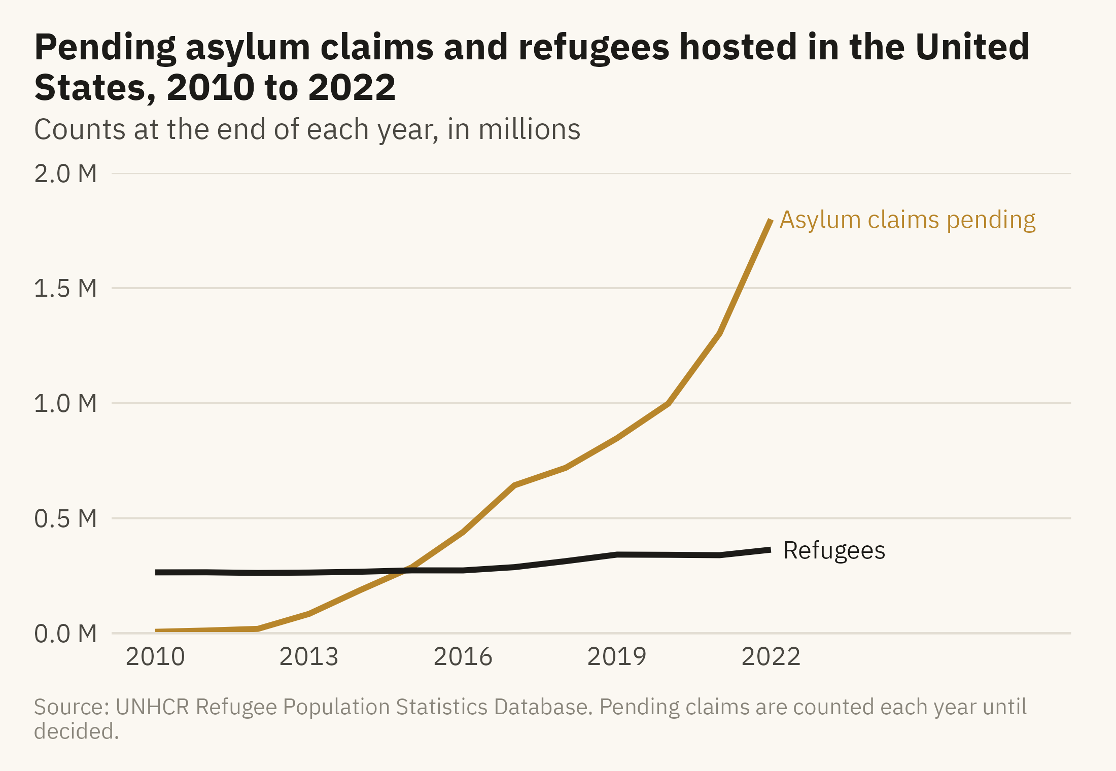
Figure 3.8 redraws the chart with three changes. The title names the unit. The refugee series is added for comparison, with both series starting from zero. The headline is replaced with a descriptive title.
Show the code
ends <- long |>filter(year ==2022)ggplot(long, aes(year, n, color = series)) +geom_line(linewidth =1) +mv_label_end(ends, aes(label = series, color = series), nudge_x =0.3) +scale_color_manual(values =c(`Refugees`= mv_ink$ink, `Asylum claims pending`=mv_accent()), guide ="none") +scale_x_continuous(breaks =seq(2010, 2022, 3), limits =c(2010, 2027)) +scale_y_continuous(labels =label_comma(scale =1e-6, suffix =" M"), limits =c(0, 2e6), expand =expansion(0)) +labs(title ="Pending asylum claims and refugees hosted in the United States, 2010 to 2022",subtitle ="Counts at the end of each year, in millions",x =NULL, y =NULL, caption =mv_source("UNHCR Refugee Population Statistics Database","Pending claims are counted each year until decided")) +theme_mv()
Figure 3.8: Pending asylum claims and refugees hosted in the United States, 2010 to 2022, with the unit stated and both series from zero. The backlog grew from 6,000 to 1.8 million. The refugee series, which the viral chart left out, grew slowly over the same years. Source: UNHCR Refugee Population Statistics Database.
The finding is unchanged. The backlog grew from about 6,000 to 1.8 million, and Figure 3.8 shows that growth. The differences from the viral chart are the stated unit, the second series, and a title that describes the data instead of stating a conclusion.
ImportantEthics Moment: The Word “Flood”
Question 1 gave the sentence “asylum seekers flooded in” as the reading most people would take from the viral chart. The word “flood” describes people as a natural force, and the data does not support that description. The word comes from the writer, not from the numbers. When a chart is about people, every word in the title and caption is a claim about those people, and readers may accept the claim because the bars are accurate. The seven questions check the numbers and the encoding. The words around the chart require a separate check, which only the reader can make.
TipTry It Online
Chart Autopsy at viz.marginoferrormedia.com/apps presents a chart drawn from a public dataset and asks you to find its problem within a time limit. The problems correspond to this chapter’s seven questions. After each round, the app redraws the chart with the problem fixed and shows how the conclusion changes. A second mode lets you paste a chart’s numbers and apply the seven questions one at a time.
WarningAI Reality Check: The Confident Caption
If the UNHCR file is given to a language model with a request for a chart of asylum seekers in the United States, the model will often produce a bar chart titled “Annual asylum seekers, 2010 to 2022.” The bars will be correct and the title will be wrong. The figure is a stock of pending claims, and the model did not consult the documentation that says so. The chart itself contains no sign of the error.
Question 1 catches this error when a reader asks it. In my experience, language models handle the encoding choices covered in Chapter 2 reasonably well. They are less reliable on the questions in this chapter, because those depend on knowing what a number means. That information is in the data documentation, and the reader has to check it.
3.10 Putting It All Together
A chart made by someone else reflects choices made by its author. The seven questions in this chapter identify those choices: what is counted, where the axis starts, what the time window is, what the denominator is, whether the encoding fits the comparison, what comparison is presented, and who made the chart and why. Checks on the axis and the encoding can be made from the chart alone. Checks on the unit, the denominator, and the comparison require knowledge of the data and its documentation. The viral chart passed the first group of checks and failed the second.
3.11 Looking Ahead
Part II covers the choice of chart. Each of its five chapters takes one question that can be asked of data: comparison, distribution, relationship, change, and place. Each chapter works through the chart forms that answer its question. Chapter 4 covers comparison and composition, using the full UNHCR data on where refugees come from and where they go. It begins with the stacked bar, a relative of the stacked area that Figure 3.7 showed to be hard to read, and states the conditions under which it is the right choice.
3.12 Further Reading and References
Cairo, A. (2019). How Charts Lie: Getting Smarter about Visual Information. W. W. Norton. A book-length treatment of the problems in this chapter.
Huff, D. (1954). How to Lie with Statistics. W. W. Norton. A short account of the truncated axis and the chosen window.
Nguyen, V. T., Jung, K., and Gupta, V. (2021). Examining data visualization pitfalls in scientific publications. Visual Computing for Industry, Biomedicine, and Art, 4, 27. A survey of how often published charts fail the checks in this chapter.
UNHCR (2023). Refugee Data Finder: Methodology. The documentation that defines refugees, asylum-seekers, and the other categories in the data, and the source of the stock-versus-flow distinction used here.
Wainer, H. (1984). How to display data badly. The American Statistician, 38(2), 137–147. A catalogue of display failures with examples.
3.13 Key Terms
Stock and flow. A stock is a count at a moment. A flow is a count over a period. The same word often names both, and a chart should say which it shows.
Time window. The start and end of the series an author chose to show. Changing it can reverse the apparent trend.
Denominator. What a count is divided by to produce a rate. A count describes the size of a group, and a rate describes that size relative to a population.
Dual axis. Two vertical scales on one chart. The relationship between the two series depends on the ratio of the scales, which the author chose.
Stacked area chart. Series drawn on top of each other. Only the bottom series and the total can be read accurately.
Provenance. Who made the chart, from what data, with what purpose.
3.14 Exercises
Check Your Understanding
Classify each as a stock or a flow: unemployment rate, new unemployment claims, national debt, annual deficit, hospital beds occupied, hospital admissions.
The viral chart’s axis starts at zero. Explain in two sentences why that does not make it an accurate chart.
Figure 3.4 shows three windows. Which of the three is the author’s best defense if challenged, and why?
In Figure 3.6, the lines cross in 2016. What would have to be true of the data for a crossing to mean something?
List the seven questions from memory, then check them against the table.
Apply It
Using ch03-us-asylum.csv, draw the pending claims series as a bar chart with the axis starting at 500,000. Measure the lie factor against the corrected version, and write one sentence a reader would take from each.
Using ch03-hosts-2022.csv, find three countries that would move more than twenty places between the count ranking and the per-capita ranking. For each, write the headline a count-based chart would support and the headline a rate-based chart would support.
Draw the eight origin countries from Figure 3.7 as a 100 percent stacked bar for 2010, 2016, and 2022. Which comparison is this chart good for, and which does it make impossible?
Find a chart in a news story from the past month. Apply the seven questions and record the answer to each. Which question found the most?
Think Deeper
The chapter argues that the questions about the unit and the comparison catch more than the questions about the axis and the encoding. Give one case where the reverse is true.
UNHCR publishes the data that the viral chart misused. Should a data publisher design its releases to make this kind of misuse harder? What would that cost the people who use the data well?
Write a caption for Figure 3.1 that would make the chart accurate without changing a single bar.