10  Uncertainty

10.1 The Number Is the Middle of a Range

A poll result is usually reported as a single number, and many readers treat that number as exact. It is an estimate from a sample. A poll of 1,000 people estimates a share with a margin of error of about three percentage points. The true share is within three points of the reported number in about nineteen samples out of twenty. A lead of two points in such a poll is inside the margin, so the poll does not establish which candidate is ahead.

The charts in the earlier chapters of this book drew each value as an exact point, line, or bar height. This chapter covers the cases in which the uncertainty around a value should be drawn as well. The case is election polling. In polling, the difference between the reported number and the range around it has been measured against election results over many cycles. FiveThirtyEight’s database contains about 20,000 polls from 1998 to 2023. For each poll it records the poll’s margin and the actual margin in the election.

10.2 One Poll, Three Ways

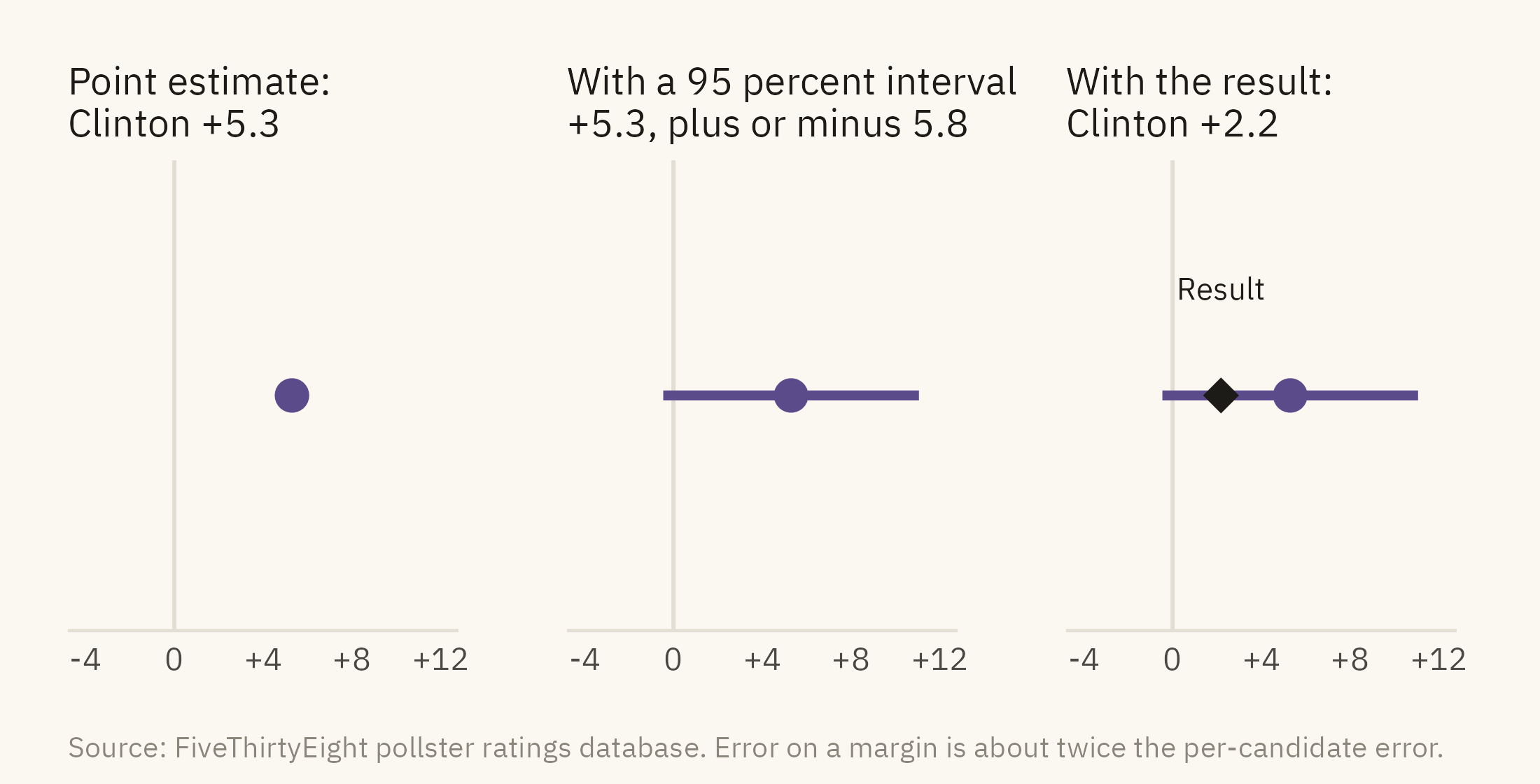
Figure 10.1 shows one poll in three forms. The poll was a national survey of 1,158 likely voters taken on October 25, 2016. It reported Clinton ahead of Trump by 5.3 points.

base <- function(title) ggplot() +
  scale_x_continuous(limits = c(-4, 12), breaks = c(-4, 0, 4, 8, 12), labels = \(x) if_else(x > 0, paste0("+", x), as.character(x))) +
  scale_y_continuous(limits = c(0.4, 1.6), breaks = NULL) +
  geom_vline(xintercept = 0, color = mv_ink$grid, linewidth = 0.5) +
  labs(x = NULL, y = NULL, title = title) + theme_mv(base_size = 10, grid = "none") + plain_title
p1 <- base(paste0("Point estimate:\n", side(m_one))) + annotate("point", x = m_one, y = 1, color = mv_accent(), size = 3.5)
p2 <- base(paste0("With a 95 percent interval:\n+", fmt1(m_one), ", plus or minus ", fmt1(e_one))) +
  annotate("segment", x = lo_one, xend = hi_one, y = 1, yend = 1, color = mv_accent(), linewidth = 1.2) +
  annotate("point", x = m_one, y = 1, color = mv_accent(), size = 3.5)
p3 <- base(paste0("With the result:\n", side(a_one))) +
  annotate("segment", x = lo_one, xend = hi_one, y = 1, yend = 1, color = mv_accent(), linewidth = 1.2) +
  annotate("point", x = m_one, y = 1, color = mv_accent(), size = 3.5) +
  annotate("point", x = a_one, y = 1, color = mv_ink$ink, shape = 18, size = 4) +
  annotate("text", x = a_one, y = 1.3, label = "Result", size = 2.8, family = mv_font(), color = mv_ink$ink)
p1 + p2 + p3 + plot_annotation(caption = mv_source(src, "Error on a margin is about twice the per-candidate error"), theme = cap_theme)

Figure 10.1: One national poll from October 2016, shown as a point (left), as a point with its 95 percent margin of error (center), and with the result added (right). The poll’s range of plus or minus 2.9 points on each candidate becomes a range of about 5.8 points on the margin. That range covers the actual margin of 2.2, so the poll was within its stated error. Only the point form, without the range, makes the poll look wrong. Source: FiveThirtyEight pollster ratings database.

The three panels lead to three different readings. From the first panel, a reader learns that Clinton led by 5.3. From the second, a reader learns that the range ran from Trump +0.5 to Clinton +11.1. The range crosses zero, so this poll on its own did not establish which candidate was ahead. From the third, a reader learns that the result fell inside the range. A reader who saw only the first panel and then saw the result might conclude that the poll had failed. The poll was within its stated error. The point form left out the range. The comparison with the result needs the range.

10.3 How Wrong Are Polls?

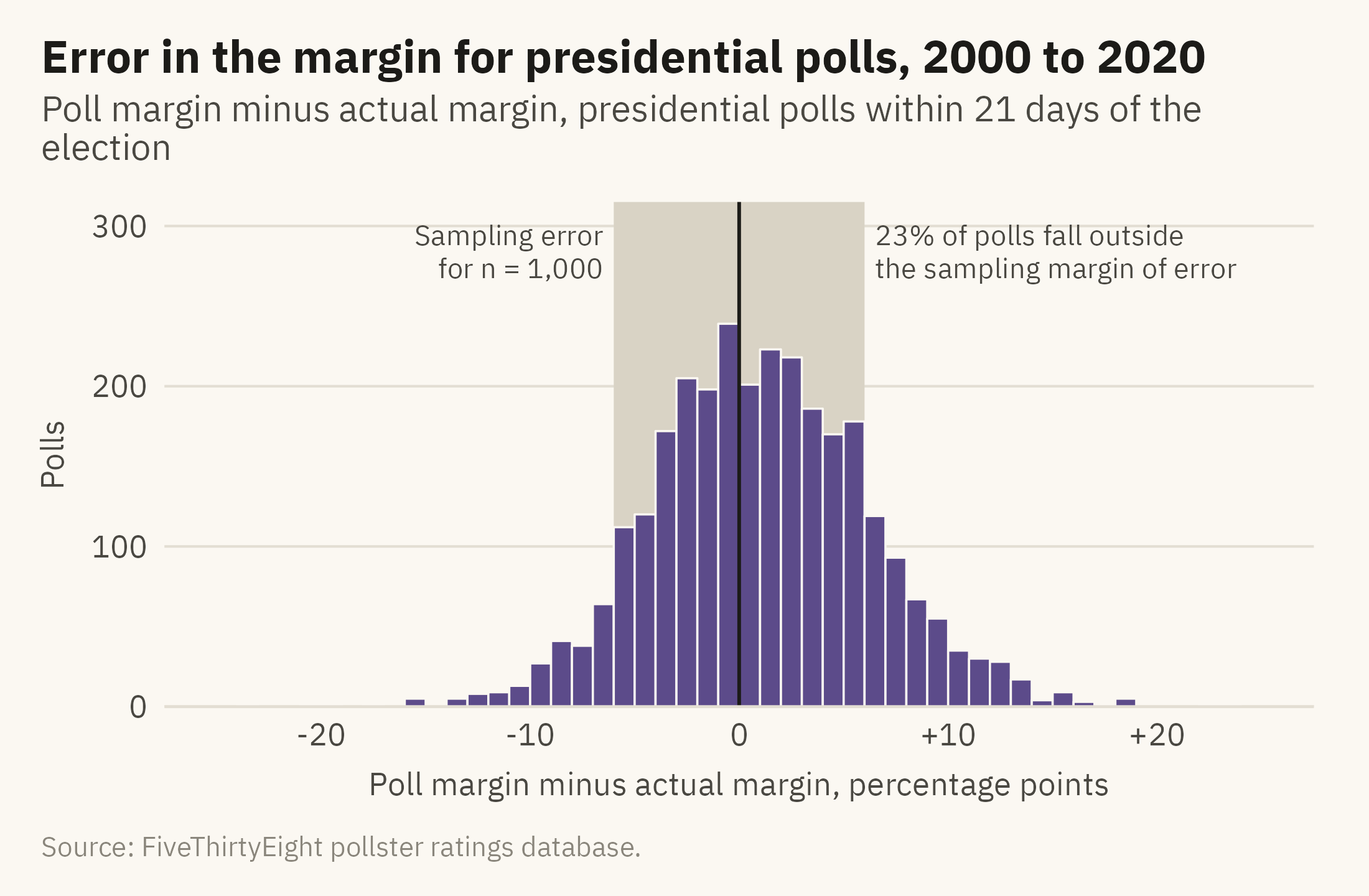
The margin of error covers sampling error only. Sampling error is the error that comes from asking 1,000 people rather than everyone. Polls have other sources of error. The people who answer a poll can differ from the people who do not. The likely-voter model is an estimate of who will vote, and it can be wrong. The wording of a question can shift the answers. Figure 10.2 shows the distribution of actual errors in presidential polls taken in the last three weeks before an election. The shaded band is the sampling margin of error for a poll of 1,000.

share_out <- mean(abs(late$error) > 6)
ggplot(late, aes(error)) +
  annotate("rect", xmin = -6, xmax = 6, ymin = 0, ymax = Inf, fill = "#D9D3C5") +
  geom_histogram(binwidth = 1, boundary = 0, fill = mv_accent(), color = mv_ink$canvas, linewidth = 0.3) +
  geom_vline(xintercept = 0, color = mv_ink$ink, linewidth = 0.5) +
  annotate("text", x = 6.5, y = 300, label = paste0(percent(share_out, 1), " of polls fall outside\nthe sampling margin of error"),
           hjust = 0, vjust = 1, size = 2.9, family = mv_font(), color = mv_ink$ink2, lineheight = 0.95) +
  annotate("text", x = -6.5, y = 300, label = "Sampling error\nfor n = 1,000", hjust = 1, vjust = 1, size = 2.9, family = mv_font(), color = mv_ink$ink2, lineheight = 0.95) +
  scale_x_continuous(limits = c(-25, 25), breaks = seq(-20, 20, 10), labels = \(x) if_else(x > 0, paste0("+", x), as.character(x))) +
  scale_y_continuous(expand = expansion(mult = c(0, 0.05))) +
  labs(title = "Error in the margin for presidential polls, 2000 to 2020",
       subtitle = "Poll margin minus actual margin, presidential polls within 21 days of the election",
       x = "Poll margin minus actual margin, percentage points", y = "Polls", caption = mv_source(src)) +
  theme_mv()

Figure 10.2: Error in the margin, poll minus result, for 2,900 presidential polls taken within 21 days of the election, 2000 to 2020. The shaded band is the sampling margin of error for a poll of 1,000, plus or minus 6 points on the margin. About a quarter of polls fall outside it. The center of the distribution is also above zero, so on average the polls overstated the Democratic candidate’s margin. Source: FiveThirtyEight pollster ratings database.

The histogram shows two findings. First, the spread of errors is wider than sampling error alone predicts. Shirani-Mehr, Rothschild, Goel, and Gelman (2018) estimated that the real error of election polls is about twice the published margin of error. Secondly, the center of the distribution is above zero. The polls in this period overstated the Democratic candidate’s margin by a few points on average. The first finding concerns random error, which averaging many polls reduces. The second concerns systematic error, which is error shared by all the polls in the same direction. When all the polls lean the same way, their average leans the same way.

10.4 Showing a Range

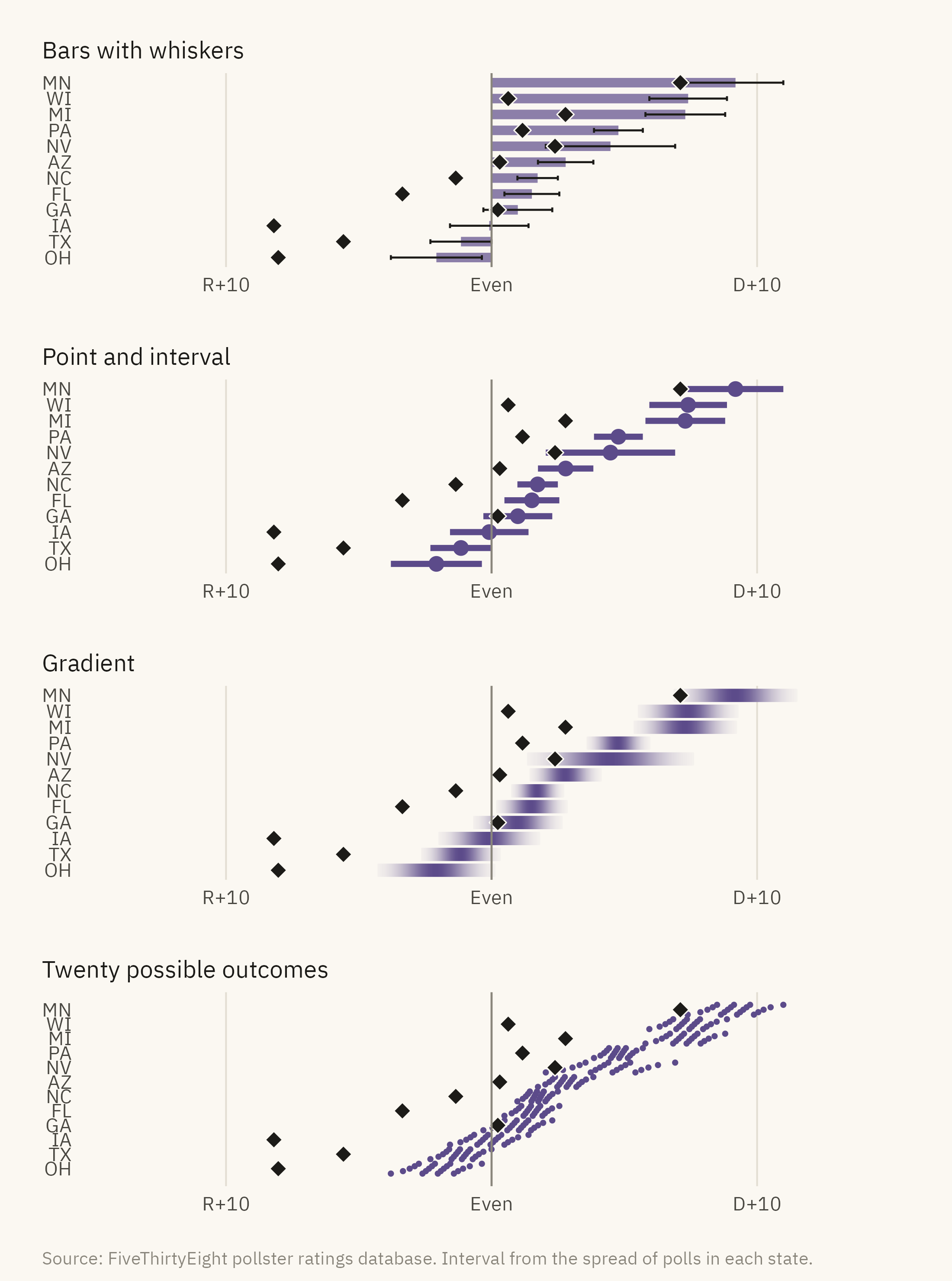
When an estimate has a range, the chart can show the range in several forms. Figure 10.3 shows four of them. The data are the final polling averages for twelve battleground states in 2020.

bg <- c("AZ", "GA", "WI", "PA", "NC", "MI", "NV", "FL", "TX", "OH", "MN", "IA")
s20 <- pres |> filter(cycle == 2020, state %in% bg, days_to_election <= 21) |>
  group_by(state) |> summarise(n = n(), est = mean(margin_poll), se = sd(margin_poll) / sqrt(n()),
                                actual = first(margin_actual), .groups = "drop") |>
  mutate(lo = est - 1.96 * se, hi = est + 1.96 * se, state = fct_reorder(state, est))
lab_x <- scale_x_continuous(limits = c(-14, 14), breaks = c(-10, 0, 10), labels = \(x) if_else(x > 0, paste0("D+", x), if_else(x < 0, paste0("R+", -x), "Even")))
# The result diamond, drawn with a thin canvas outline so it stays visible over bars and gradients
result_pt <- geom_point(data = s20, aes(actual, state), shape = 23, size = 2.4, fill = mv_ink$ink, color = mv_ink$canvas, stroke = 0.4)
f1 <- ggplot(s20, aes(est, state)) +
  geom_col(fill = mv_accent(), width = 0.6, alpha = 0.7) +
  geom_errorbar(aes(xmin = lo, xmax = hi), width = 0.3, color = mv_ink$ink, linewidth = 0.4) +
  result_pt +
  geom_vline(xintercept = 0, color = mv_ink$mute, linewidth = 0.4) + lab_x +
  labs(x = NULL, y = NULL, title = "Bars with whiskers") + theme_mv(base_size = 10, grid = "x") + plain_title
f2 <- ggplot(s20, aes(est, state)) +
  geom_segment(aes(x = lo, xend = hi, yend = state), color = mv_accent(), linewidth = 1.2) +
  geom_point(color = mv_accent(), size = 2.4) +
  result_pt +
  geom_vline(xintercept = 0, color = mv_ink$mute, linewidth = 0.4) + lab_x +
  labs(x = NULL, y = NULL, title = "Point and interval") + theme_mv(base_size = 10, grid = "x") + plain_title
grad <- s20 |> crossing(k = seq(-2.5, 2.5, length.out = 201)) |>
  mutate(x = est + k * se, w = dnorm(k) / dnorm(0),
         fill = colorRampPalette(c(mv_ink$canvas, mv_accent()))(101)[round(w * 100) + 1])
f3 <- ggplot(grad, aes(x, state)) +
  geom_tile(aes(fill = fill, color = fill, width = 5 * se / 200), height = 0.75, linewidth = 0.25) +
  scale_fill_identity() + scale_color_identity() +
  result_pt +
  geom_vline(xintercept = 0, color = mv_ink$mute, linewidth = 0.4) + lab_x +
  labs(x = NULL, y = NULL, title = "Gradient") + theme_mv(base_size = 10, grid = "x") + plain_title
# Twenty quantiles per state, stacked in five rows in order of value so neighbouring dots do not overlap
qd <- s20 |> crossing(i = 1:20) |> mutate(q = (i - 0.5) / 20, x = qnorm(q, est, se), row = ((i - 1) %% 5 - 2) * 0.17)
f4 <- ggplot(qd, aes(x, as.numeric(state) + row)) +
  geom_point(color = mv_accent(), size = 0.55) +
  scale_y_continuous(breaks = seq_along(levels(s20$state)), labels = levels(s20$state), limits = c(0.4, 12.6)) +
  geom_point(data = s20, aes(actual, as.numeric(state)), shape = 23, size = 2.4, fill = mv_ink$ink, color = mv_ink$canvas, stroke = 0.4) +
  geom_vline(xintercept = 0, color = mv_ink$mute, linewidth = 0.4) + lab_x +
  labs(x = NULL, y = NULL, title = "Twenty possible outcomes") + theme_mv(base_size = 10, grid = "x") + plain_title
f1 / f2 / f3 / f4 + plot_annotation(caption = mv_source(src, "Interval from the spread of polls in each state"), theme = cap_theme)

Figure 10.3: Four ways to show the same uncertainty. The average poll margin in twelve states in the last three weeks of 2020, with a 95 percent interval from the spread of polls, shown as a bar with error whiskers, a point with an interval, a gradient that fades with distance from the estimate, and a quantile dot plot in which each of twenty dots is an equally likely outcome. The dots are stacked in five rows so that they can be counted. The actual result is the black diamond. Source: FiveThirtyEight pollster ratings database.

The four forms differ in how accurately readers judge them. Bars with whiskers are the most common form and the least accurate. The bar extends from zero to the estimate, so a reader sees the full length as the value and the whiskers as a detail. Correll and Gleicher (2014) found that readers judge values inside the bar as more likely than values outside it at the same distance from the estimate. The two values are equally likely. The point with an interval has no bar, and readers do not make this error with it. The gradient shows that the probability of an outcome decreases with distance from the estimate rather than ending at a boundary. Its drawback is that there is no edge for a reader to read a value from. The quantile dot plot shows the range as a set of dots, each an equally likely outcome. In Iowa, 11 of the twenty dots fall on the Republican side of zero and 9 on the Democratic side. Kay, Kola, Hullman, and Munson (2016) found that readers estimate probabilities more accurately from counts of dots than from a continuous density curve.

The diamonds mark the results. In most of these states, the result fell at the edge of the interval or beyond it, and in every case on the same side. This is the systematic error in Figure 10.2, shown one state at a time.

10.5 Uncertainty Over Time

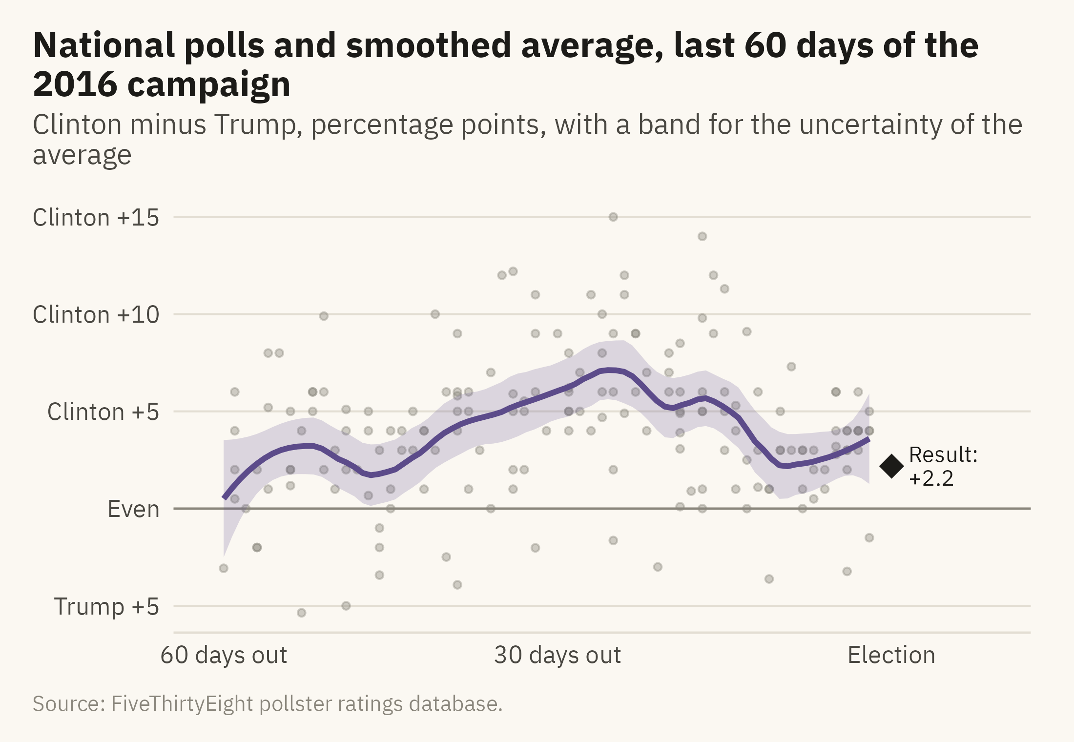
A poll average over a campaign is usually drawn as a line. A line alone does not show the uncertainty in the average. Figure 10.4 shows the 2016 national polls and the average with its band.

n16 <- pres |> filter(race == "2016_Pres-G_US", days_to_election <= 70)
ggplot(n16, aes(-days_to_election, margin_poll)) +
  geom_hline(yintercept = 0, color = mv_ink$mute, linewidth = 0.4) +
  geom_point(color = mv_ink$mute, size = 1, alpha = 0.4) +
  geom_smooth(method = "loess", span = 0.3, color = mv_accent(), fill = mv_accent(), alpha = 0.2, linewidth = 1, formula = y ~ x) +
  annotate("point", x = 0, y = a_one, shape = 18, size = 4, color = mv_ink$ink) +
  annotate("text", x = 1.5, y = a_one, label = paste0("Result:\n+", fmt1(a_one)), hjust = 0, vjust = 0.5, size = 2.9, family = mv_font(), color = mv_ink$ink, lineheight = 0.9) +
  scale_x_continuous(breaks = c(-60, -30, 0), labels = c("60 days out", "30 days out", "Election"), limits = c(-61, 9)) +
  scale_y_continuous(breaks = seq(-5, 15, 5), labels = \(x) if_else(x > 0, paste0("Clinton +", x), if_else(x < 0, paste0("Trump +", -x), "Even"))) +
  labs(title = "National polls and smoothed average, last 60 days of the 2016 campaign",
       subtitle = "Clinton minus Trump, percentage points, with a band for the uncertainty of the average",
       x = NULL, y = NULL, caption = mv_source(src)) +
  theme_mv()

Figure 10.4: National presidential polls in the last 60 days of the 2016 campaign (grey points), a smoothed average (line), and a band for the uncertainty in the average. The band is the uncertainty of the average, not the range where a single poll might fall. The result, Clinton by 2.2, is marked. Source: FiveThirtyEight pollster ratings database.

The band around an average is narrow because many polls went into the average. The band shows the uncertainty in the average itself. It does not show where the next poll will fall, and it does not show where the result will fall. The spread of the grey points shows where a single poll might fall. The history of systematic error across past elections is the only guide to where the result might fall. The polls from one cycle do not contain that history, so the caption has to state the distinction.

10.6 The Hidden Variable: Sample Size

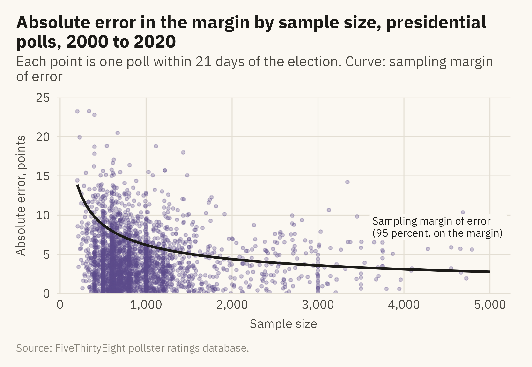
A poll’s stated margin of error is computed from its sample size. Figure 10.5 compares that stated margin with the actual errors. Each point is one poll, placed by its sample size and the absolute size of its error. The curve is the sampling margin of error at each sample size.

curve <- tibble(n = seq(200, 5000, 50), e = 2 * moe(n))
ggplot(samp, aes(sample_size, abs(error))) +
  geom_point(color = mv_accent(), size = 0.9, alpha = 0.3) +
  geom_line(data = curve, aes(n, e), color = mv_ink$ink, linewidth = 0.9) +
  annotate("label", x = 3600, y = 8.5, label = "Sampling margin of error\n(95 percent, on the margin)", hjust = 0, size = 2.8,
           family = mv_font(), color = mv_ink$ink, fill = mv_ink$canvas, label.size = 0, lineheight = 0.95) +
  scale_x_continuous(labels = label_comma()) +
  scale_y_continuous(limits = c(0, 25), expand = expansion(0)) +
  labs(title = "Absolute error in the margin by sample size, presidential polls, 2000 to 2020",
       subtitle = "Each point is one poll within 21 days of the election. Curve: sampling margin of error",
       x = "Sample size", y = "Absolute error, points", caption = mv_source(src)) +
  theme_mv(grid = "y") + theme(panel.grid.major.x = element_line(color = mv_ink$grid, linewidth = 0.35))

Figure 10.5: Absolute error in the margin against sample size for presidential polls within 21 days of the election, with samples of 200 to 5,000, and the sampling margin of error on the margin drawn as a curve. The curve falls steeply below 500 respondents and flattens after that. The typical error of the polls falls only a little as samples grow. The share of polls above the curve rises with sample size, from about 12 percent below 500 respondents to about 61 percent above 3,000. Source: FiveThirtyEight pollster ratings database.

10.7 Errors in the Same Direction

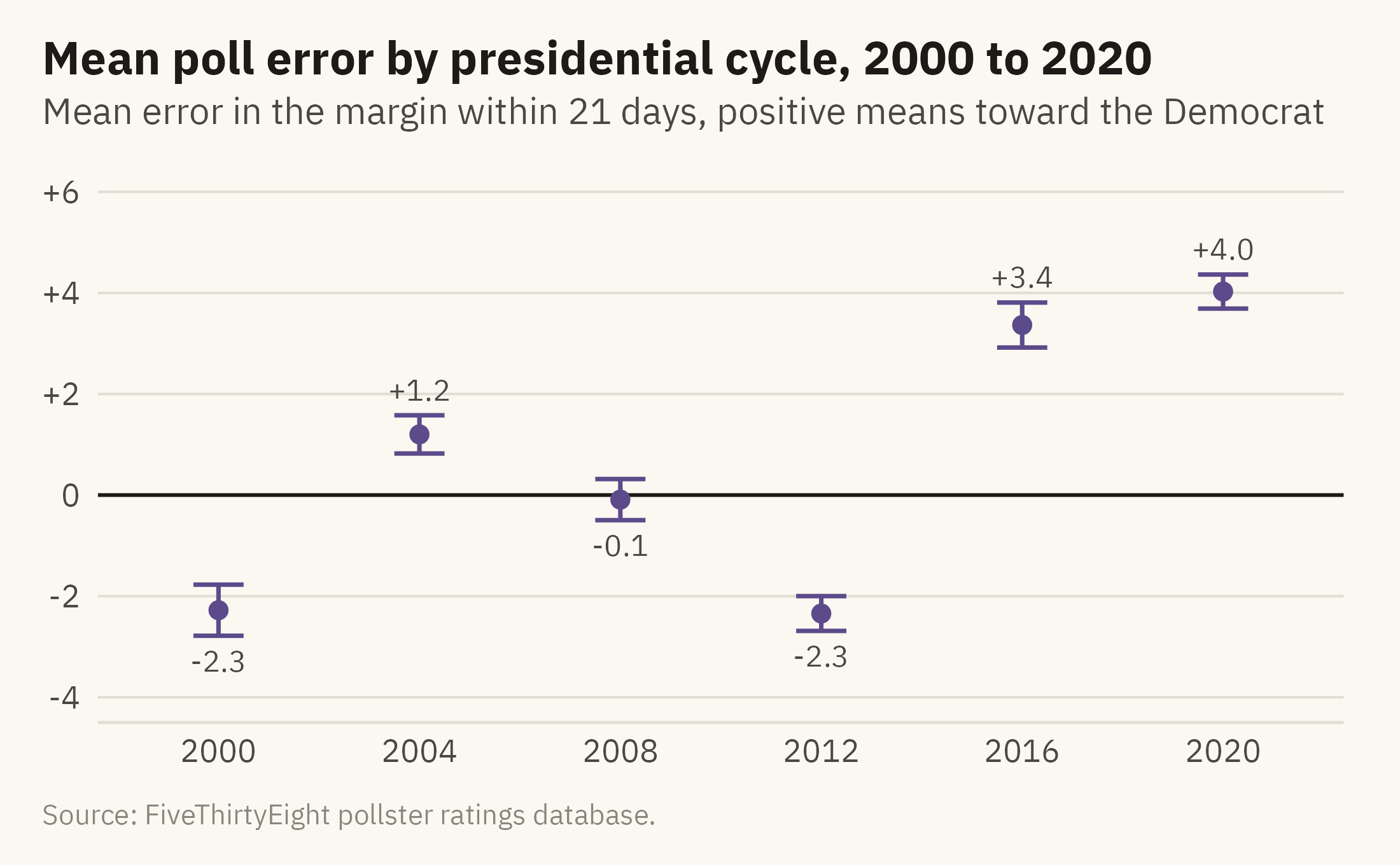
Systematic error is the part of the error that averaging does not remove. Figure 10.6 shows the mean error in the final three weeks of each presidential cycle, with a 95 percent interval for each mean.

lean <- late |> group_by(cycle) |> summarise(n = n(), m = mean(error), se = sd(error) / sqrt(n()), .groups = "drop") |>
  mutate(lo = m - 1.96 * se, hi = m + 1.96 * se)
ggplot(lean, aes(factor(cycle), m)) +
  geom_hline(yintercept = 0, color = mv_ink$ink, linewidth = 0.5) +
  geom_errorbar(aes(ymin = lo, ymax = hi), color = mv_accent(), width = 0.25, linewidth = 0.6) +
  geom_point(color = mv_accent(), size = 2) +
  geom_text(aes(label = sprintf("%+.1f", m), y = if_else(m > 0, hi + 0.5, lo - 0.5)), size = 3, family = mv_font(), color = mv_ink$ink2) +
  scale_y_continuous(limits = c(-4, 6), breaks = seq(-4, 6, 2), labels = \(x) if_else(x > 0, paste0("+", x), as.character(x))) +
  labs(title = "Mean poll error by presidential cycle, 2000 to 2020",
       subtitle = "Mean error in the margin within 21 days, positive means toward the Democrat",
       x = NULL, y = NULL, caption = mv_source(src)) +
  theme_mv()

Figure 10.6: Mean error in the margin, poll minus result, across presidential polls in the final 21 days of each cycle from 2000 to 2020, with 95 percent intervals. A positive value means polls leaned toward the Democrat. The lean changes sign across cycles and was largest in 2016 and 2020. Source: FiveThirtyEight pollster ratings database.

The intervals are narrow because each cycle contains hundreds of polls. The means are well away from zero in most cycles, which is the pattern that systematic error produces. The direction of the lean changes from cycle to cycle. It reversed between 2012 and 2016. A chart of the most recent cycle alone would not show this, so a reader could not tell from it which direction the next cycle’s polls might lean.

ImportantEthics Moment: Precision Is a Claim

A chart that draws a poll as a point implies more precision than the poll has. A headline that says “Clinton leads by 5” when the range runs from Trump +0.5 to Clinton +11.1 implies the same precision in words. Neither is false. Both leave out the part of the finding that would weaken the story. Voters, donors, and candidates who rely on the story may act as if the number were more precise than it is. Showing the range reports the finding in full. The number alone is a summary, and the range is the part that the summary leaves out.

TipTry It Online

Give or Take at viz.marginoferrormedia.com/apps lets you set a sample size and a true margin, draw a poll, and see the interval. A second tab draws a hundred polls at once and counts how many intervals cover the truth. A third adds a systematic lean and shows why a hundred polls with the same lean agree with each other and miss the result.

WarningAI Reality Check: The Interval the Model Leaves Out

Ask a language model for a chart of poll results, and the first draft will usually show the point estimates with no intervals. Ask for the margin of error, and the draft will usually add symmetric whiskers computed from the sampling formula. As this chapter showed, the sampling formula covers about half of the real error. The model follows common newsroom practice, and that practice understates the error.

Ask for the interval. Then ask what the interval is based on, and whether it reflects sampling alone or the history of how polls like this one have missed. The history is the larger part of the error. The model can include it only if that history is in the data you gave it.

10.8 Putting It All Together

A number from a sample is the middle of a range, and a chart of that number can show the range. The margin of error covers sampling error only. The real range is wider, and the history of past misses is the only guide to how much wider. A range can be drawn as a point with an interval, a gradient, or a set of equally likely outcomes. Bars with whiskers lead readers to misjudge the interval, so the other forms are preferred. When an average is drawn with its band, the caption should say what the band covers. Systematic error is the error that all the polls share. Averaging does not remove it, and in a close election it can be larger than the margin between the candidates.

10.9 Looking Ahead

Part IV covers the presentation of charts to an audience. Chapter 11 covers interactivity and dashboards, in which the reader controls the view. It describes what a reader gains and loses when a chart is no longer a fixed picture. The case is the services a county offers its residents, and whether a dashboard can show where the gaps in those services are.

10.10 Further Reading and References

Correll, M., and Gleicher, M. (2014). Error bars considered harmful: Exploring alternate encodings for mean and error. IEEE Transactions on Visualization and Computer Graphics, 20(12), 2142–2151. The experiments on how readers misjudge bars with whiskers.

Hullman, J., Resnick, P., and Adar, E. (2015). Hypothetical outcome plots outperform error bars and violin plots for inferences about reliability of variable ordering. PLOS ONE, 10(11), e0142444. The first study of showing uncertainty as a set of possible outcomes.

Kay, M., Kola, T., Hullman, J. R., and Munson, S. A. (2016). When (ish) is my bus? User-centered visualizations of uncertainty in everyday, mobile predictive systems. Proceedings of CHI 2016, 5092–5103. The quantile dot plot.

Shirani-Mehr, H., Rothschild, D., Goel, S., and Gelman, A. (2018). Disentangling bias and variance in election polls. Journal of the American Statistical Association, 113(522), 607–614. The study that measured the real error of polls against the sampling error, and the source of the “about twice” rule of thumb.

Silver, N. (2023). The Polls Are Still Fine. Here’s Why. FiveThirtyEight. The pollster ratings methodology and the database used throughout this chapter.

10.11 Key Terms

Margin of error. The range around a sample estimate that covers the true value most of the time, from sampling alone.

Systematic error. Error shared by all polls in the same direction. Averaging does not remove it.

Point with interval. The estimate as a dot and the range as a line. The most common form recommended for showing uncertainty.

Quantile dot plot. A set of equally likely outcomes drawn as dots, so that probability is read as a count.

Uncertainty of the average. The band around a smoothed line. It narrows with more polls and does not predict the next poll or the result.

10.12 Exercises

Check Your Understanding

1. A poll of 800 people shows a candidate at 48 percent. State the sampling margin of error and the range it implies for the share and for the margin.
2. Why is the real error of polls larger than the sampling margin of error? Name two sources.
3. In Figure 10.3, why do bars with whiskers mislead in a way that points with intervals do not?
4. Explain, in one sentence each, what the band in Figure 10.4 does and does not tell a reader.
5. What does it mean that the intervals in Figure 10.6 are narrow and the means are not near zero?

Apply It

6. Using ch10-polls.csv, draw the error histogram for Senate polls instead of presidential ones. Is the spread wider or narrower? Does it lean?
7. Build a quantile dot plot for one state in 2024 from its final three weeks of polls. Count how many of the twenty dots fall on each side of zero and write the sentence that count supports.
8. Draw the 2020 national poll average with its band and mark the result. How many days before the election did the band last include the result?
9. Compute the share of polls whose sampling interval covered the actual margin, by cycle. A well-calibrated interval would cover 95 percent. What do you find?

Think Deeper

10. The chapter describes bars with whiskers as the least accurate form, and they remain the most common. Propose two reasons that are not about accuracy.
11. A newsroom wants one number for a headline. Write a rule for when a poll’s number may stand alone and when the range must appear in the headline itself.
12. Systematic error reversed sign between 2012 and 2016. What would a chart need to show so that a reader in 2024 drew the right lesson from both?