Every year since 1970, the Census of Jails and the surveys that followed it have counted the people held in county jails on a single day. Since 1983, the National Corrections Reporting Program has counted the people held in state prisons. The Vera Institute of Justice joined the two into one dataset by county. This chapter uses that dataset to answer four questions about change over time. What changed, when did it change, how fast did it change, and how does the change compare with something else?
Jail and prison are different things. A jail is a county facility. It holds people who are waiting for trial or serving sentences under a year. A prison is a state or federal facility for longer sentences. Both counts rose from the late 1970s to 2008. The jail count peaked in 2008 and has stayed below that level since. The prison count peaked in 2008, held level for two years, and then fell slowly. Each section of this chapter takes one part of that history and shows how to chart it. One section covers the year after which the data are no longer complete.
7.2 The Line Chart
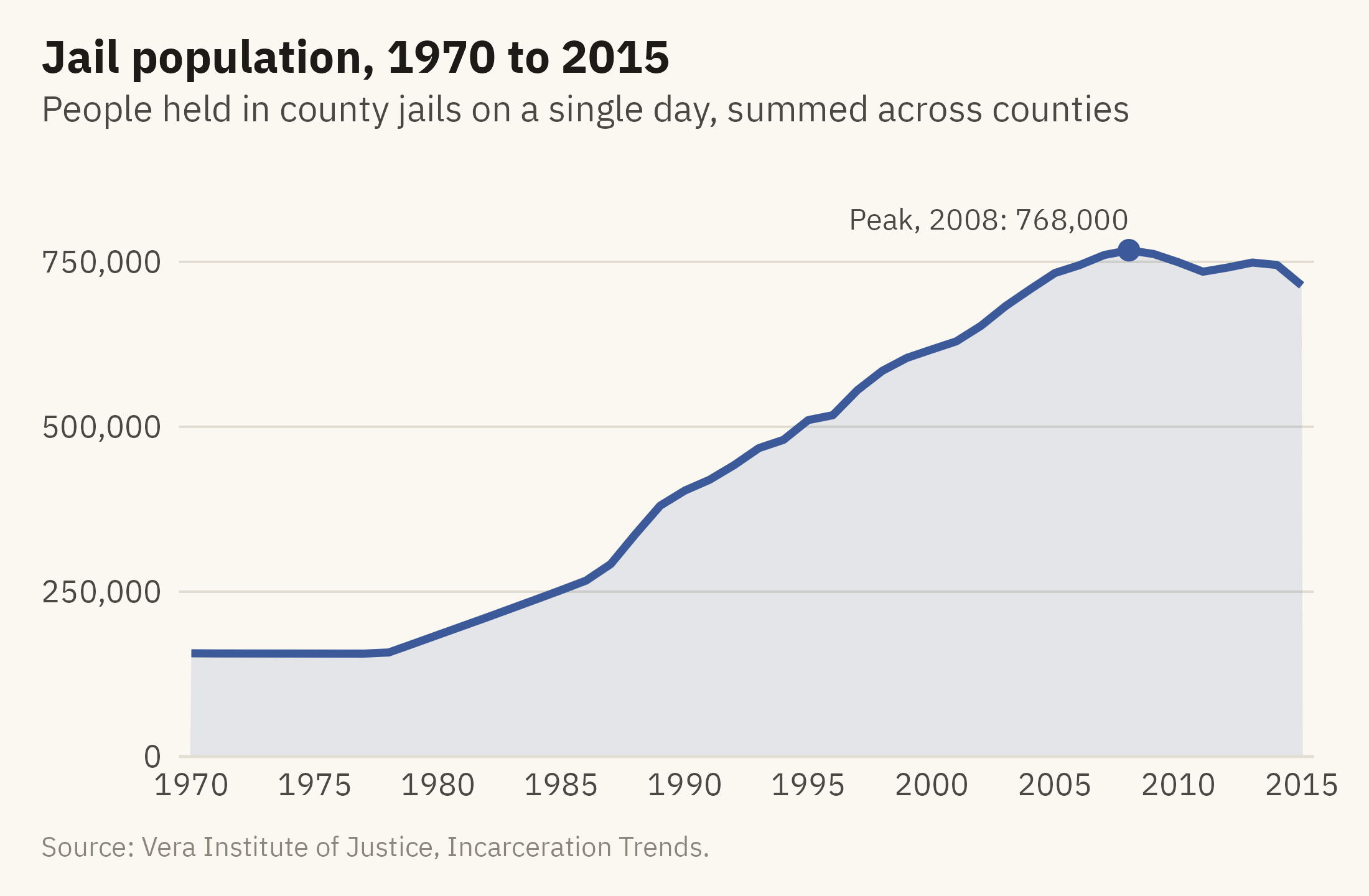
A line chart connects measurements of one quantity over time. The connection uses the Gestalt principle of connection from Chapter 2. Marks joined by a line are seen as one object, so a reader sees the series as one quantity changing rather than as separate observations. Figure 7.1 shows the jail population from 1970 to 2015.
Show the code
peak <- jail |>slice_max(jail, n =1)ggplot(jail, aes(year, jail)) +geom_area(fill =mv_accent(), alpha =0.12) +geom_line(color =mv_accent(), linewidth =1.1) +geom_point(data = peak, color =mv_accent(), size =2.4) +annotate("text", x = peak$year, y = peak$jail, label =paste0("Peak, ", peak$year, ": ", label_comma()(round(peak$jail, -3))),vjust =-1, hjust =1, size =3, family =mv_font(), color = mv_ink$ink2) +scale_x_continuous(breaks =seq(1970, 2015, 5), expand =expansion(mult =0.01)) +scale_y_continuous(labels =label_comma(), limits =c(0, 900000), expand =expansion(0)) +labs(title ="Jail population, 1970 to 2015",subtitle ="People held in county jails on a single day, summed across counties",x =NULL, y =NULL, caption =mv_source(src)) +theme_mv()
Figure 7.1: People held in county jails on a single day each year, 1970 to 2015, summed across about 3,070 counties. The count was flat through the 1970s, tripled between 1980 and 2000, and peaked in 2008. It has stayed below the peak since, with a small rise in 2012 and 2013. Source: Vera Institute of Justice, Incarceration Trends.
Three conventions in this chart apply to nearly every line chart. Time runs from left to right. The vertical axis starts at zero, because a reader sees the shaded area under the line as an amount. The peak is marked and labeled, so a reader does not have to search for it.
The zero rule is less strict for lines than for bars, because a line encodes position rather than length. A series whose values stay far from zero, such as life expectancy between 65 and 85 years, can be drawn on an axis that starts above zero. The deciding condition is whether the reader is expected to compare sizes. In Figure 7.1 the reader is, because the area under the line is shaded and the text describes a tripling, so the axis starts at zero. If the only question were the year of the peak, the axis could start higher, provided the axis labels show where it starts.
7.3 Count or Rate
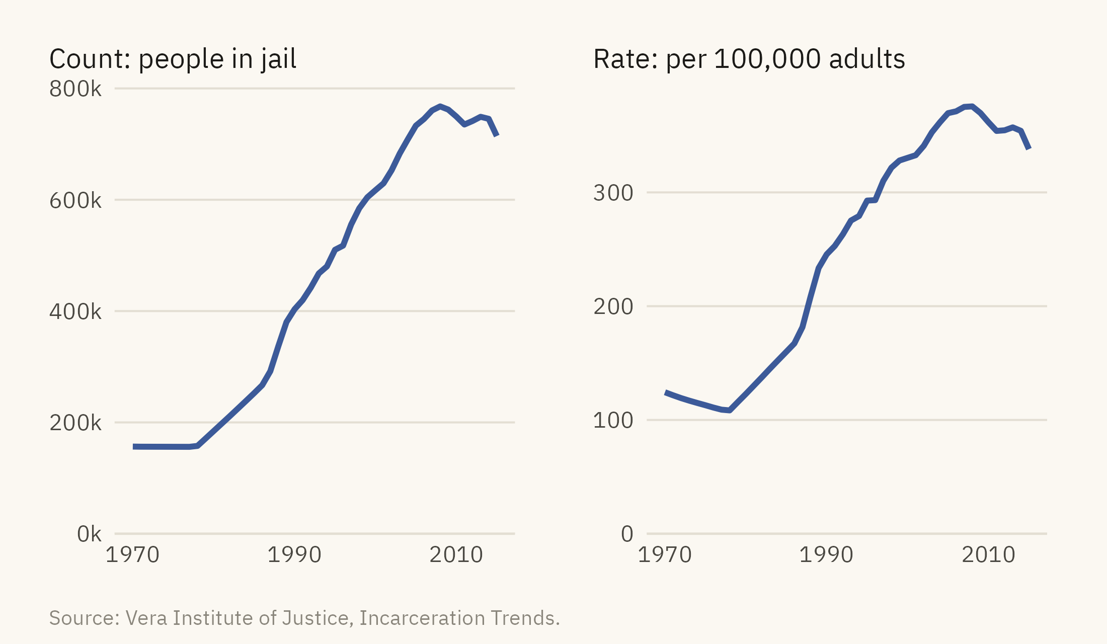
The jail count rose by a factor of 3.3 between 1980 and 2000. Over the same years, the population of adults aged 15 to 64 grew by about a quarter. A count combines growth in the thing measured with growth in the population it is drawn from. A rate divides the count by that population and removes the second part. Figure 7.2 shows both the count and the rate.
Figure 7.2: The jail count (left) and the jail rate per 100,000 residents aged 15 to 64 (right), 1970 to 2015. The rate rose almost as fast as the count, so most of the rise in the count is not explained by growth in the population. A chart of counts should be checked against the rate before a reader draws a conclusion. Source: Vera Institute of Justice, Incarceration Trends.
The two panels have the same shape. Between 1980 and 2000 the count rose by a factor of 3.3 and the rate by a factor of 2.7. The adult population grew by about a quarter over the same years, which accounts for the difference between the two factors. Most of the rise in the count is a rise in the share of adults held in jail, not a rise in the number of adults. When a count and its rate differ in shape, the change in the base explains the difference, and the rate is the better chart. When they agree, as they do here, either can be shown. The rate is still needed when places of different sizes are compared.
7.4 Two Series, One Chart
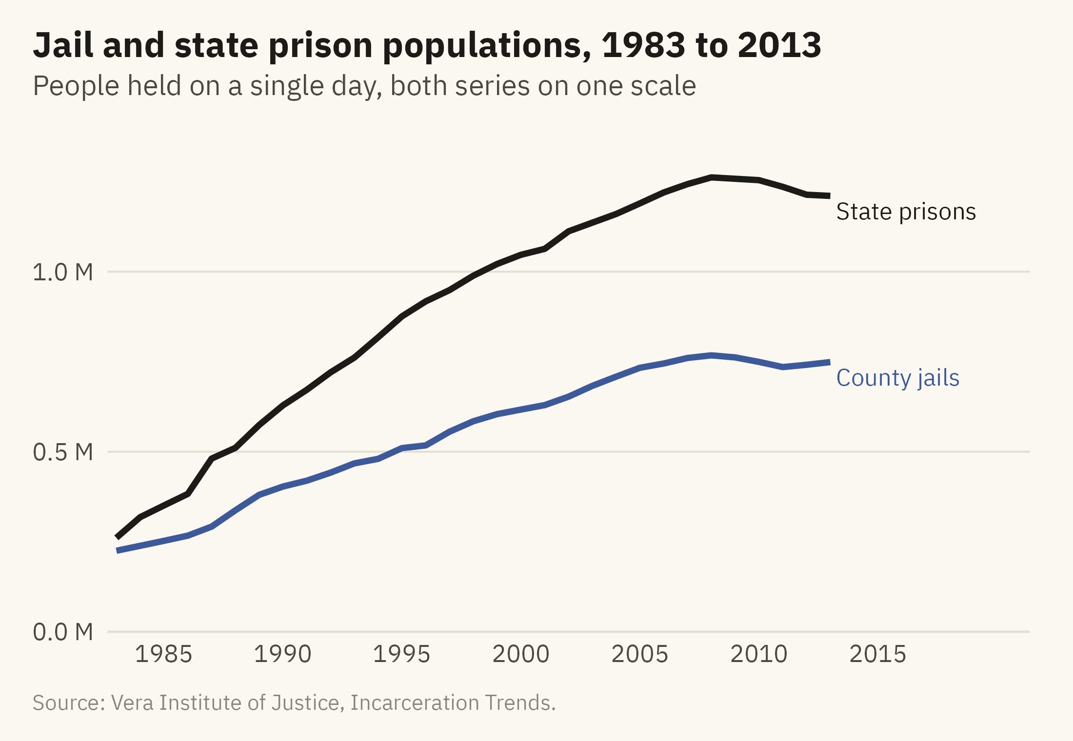
The prison count begins in 1983. The two counts can be compared by placing them on one chart. A common way to do this is a dual-axis chart, and Chapter 3 described its problems. Figure 7.3 instead uses one axis, starts both series from zero, and labels each line at its end.
Show the code
two <-bind_rows(jail |>filter(year >=1983, year <=2013) |>transmute(year, series ="County jails", n = jail), prison |>transmute(year, series ="State prisons", n = prison))ends <- two |>group_by(series) |>slice_max(year, n =1)ggplot(two, aes(year, n, color = series)) +geom_line(linewidth =1.1) +mv_label_end(ends, aes(label = series, color = series), nudge_x =0.4) +scale_color_manual(values =c(`County jails`=mv_accent(), `State prisons`= mv_ink$ink), guide ="none") +scale_x_continuous(breaks =seq(1985, 2015, 5), limits =c(1983, 2021), expand =expansion(mult =0.01)) +scale_y_continuous(labels =label_comma(scale =1e-6, accuracy =0.1, suffix =" M"), limits =c(0, 1.4e6), expand =expansion(0)) +labs(title ="Jail and state prison populations, 1983 to 2013",subtitle ="People held on a single day, both series on one scale",x =NULL, y =NULL, caption =mv_source(src)) +theme_mv()
Figure 7.3: Jail and state prison populations, 1983 to 2013, on one scale. Prison grew faster and further. Both series peaked in 2008. Jail has stayed below its peak since. Prison held level through 2010 and then came down slowly. Both series end in 2013 because county coverage drops after that, as the next figure shows. Source: Vera Institute of Justice, Incarceration Trends.
A label at the end of each line replaces the legend. The reader does not have to look away from the data to match a color to a name. Direct labels work for up to four or five series. With more series than that, small multiples are usually easier to read.
7.5 Indexing to a Start
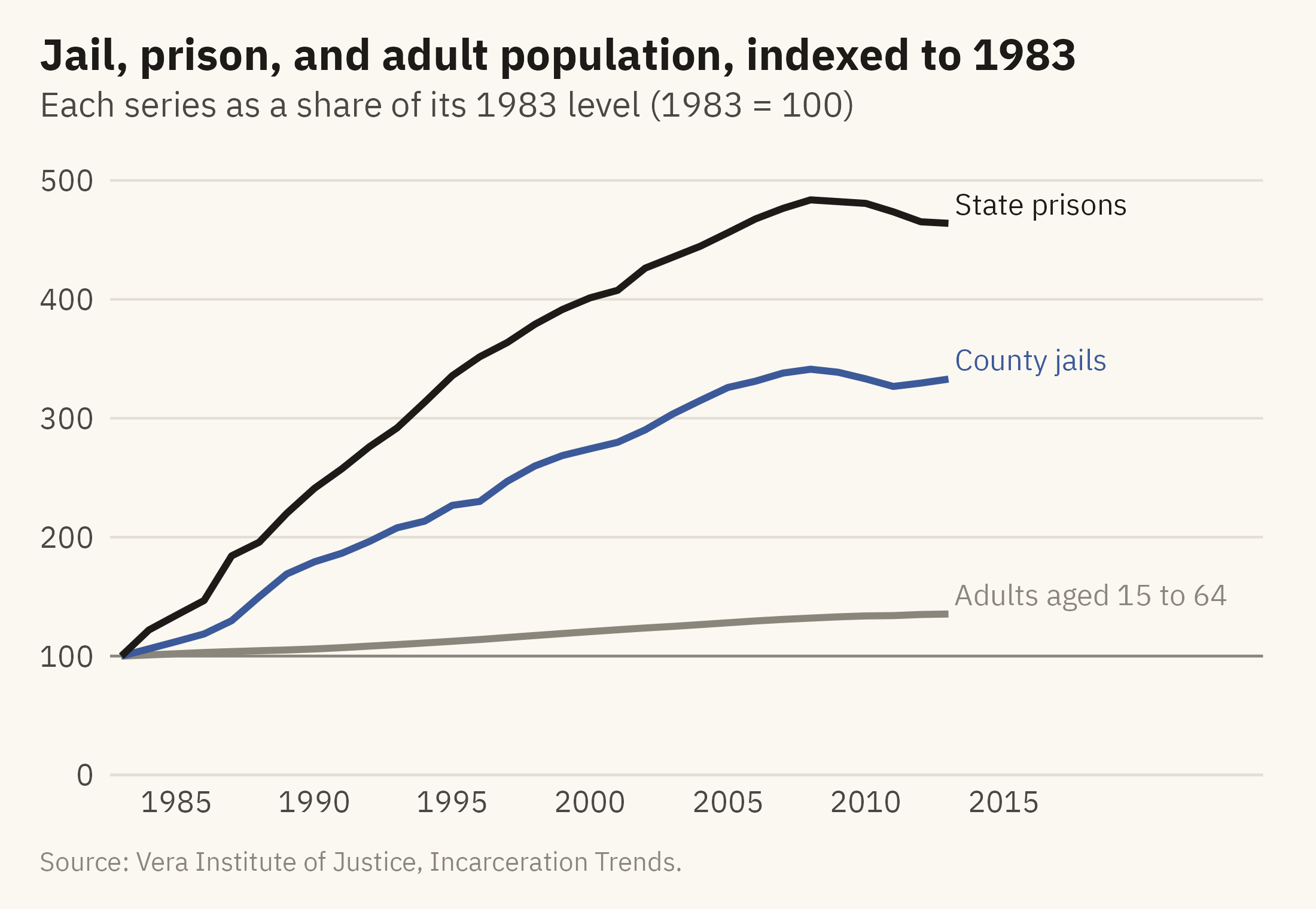
When series differ in size, their growth rates are hard to compare on one scale. The jail line in Figure 7.3 looks flatter than the prison line, partly because its values are lower. An index chart divides each series by its value in a base year. Every line then starts at 100, and a reader can compare growth rates from the slopes. Figure 7.4 indexes the jail population, the prison population, and the adult population to 1983.
Show the code
idx <- nat |>filter(year >=1983, year <=2013) |>transmute(year, `State prisons`= prison / prison[year ==1983] *100,`County jails`= jail / jail[year ==1983] *100,`Adults aged 15 to 64`= pop_15to64 / pop_15to64[year ==1983] *100) |>pivot_longer(-year, names_to ="series", values_to ="index")iend <- idx |>filter(year ==2013)ggplot(idx, aes(year, index, color = series)) +geom_hline(yintercept =100, color = mv_ink$mute, linewidth =0.4) +geom_line(linewidth =1) +mv_label_end(iend, aes(label = series, color = series), nudge_x =0.4) +scale_color_manual(values =c(`State prisons`= mv_ink$ink, `County jails`=mv_accent(), `Adults aged 15 to 64`= mv_ink$mute), guide ="none") +scale_x_continuous(breaks =seq(1985, 2015, 5), limits =c(1983, 2024), expand =expansion(mult =0.01)) +scale_y_continuous(limits =c(0, 520), expand =expansion(0)) +labs(title ="Jail, prison, and adult population, indexed to 1983",subtitle ="Each series as a share of its 1983 level (1983 = 100)",x =NULL, y =NULL, caption =mv_source(src)) +theme_mv()
Figure 7.4: Jail population, prison population, and adult population, each as a share of its 1983 value. By 2008, the prison population was 4.8 times its 1983 level and the jail population 3.4 times, while the adult population grew by a third. Source: Vera Institute of Justice, Incarceration Trends.
An index chart leaves out the levels. A reader cannot tell from Figure 7.4 that prisons hold more people than jails. The chart shows only that the prison population grew faster. When the levels matter, the index can be shown beside a chart of the levels, or the levels can be stated in the caption. The choice of base year also changes what the chart shows. If the base year is a low point, every later value appears as growth. If the base year is a peak, every later value appears as decline.
7.6 Where the Data Stops
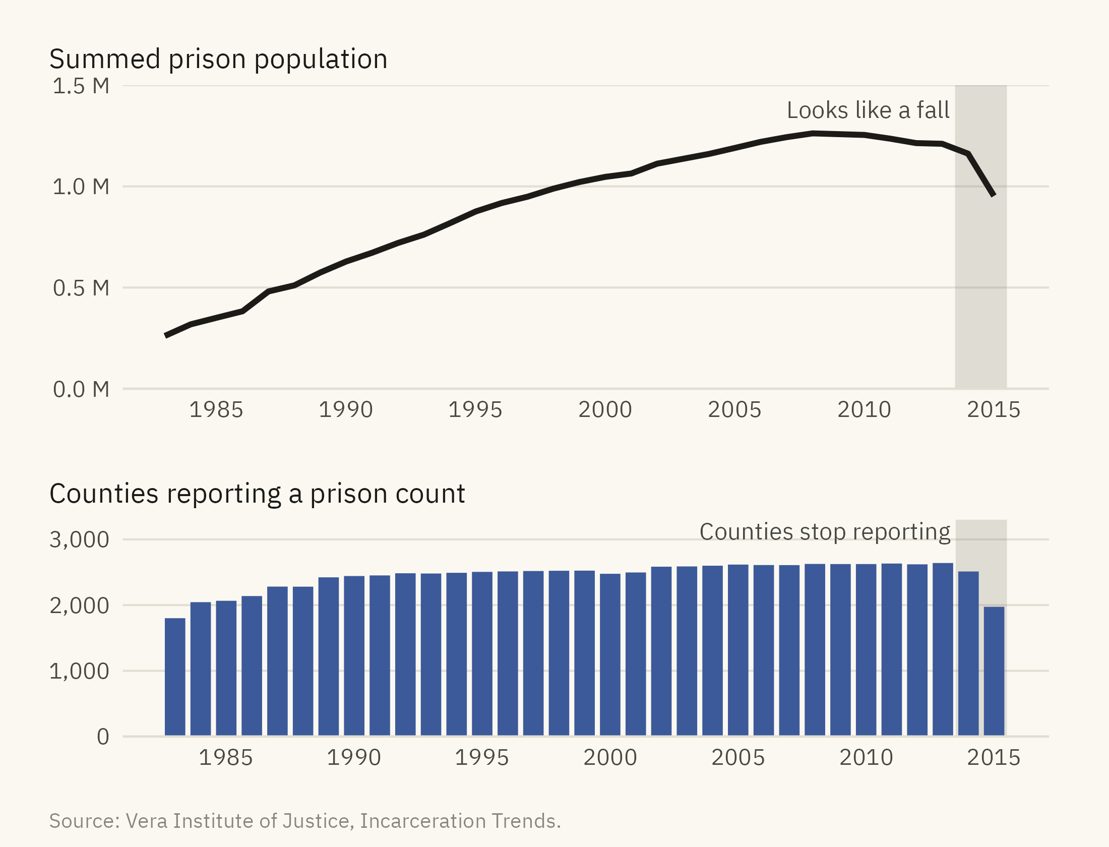
Figure 7.3 ends the prison series at 2013 because county coverage falls after that year. Vera’s prison counts come from county-level records, and not every state reports every year. About 130 counties are missing in 2014 and about 670 in 2015. A sum across the reporting counties therefore falls by about a fifth between 2013 and 2015, although the number of people in prison did not. Figure 7.5 shows the summed series with the number of reporting counties beneath it.
Show the code
cov <- nat |>filter(year >=1983)top <-ggplot(cov, aes(year, prison)) +annotate("rect", xmin =2013.5, xmax =2015.5, ymin =0, ymax =Inf, fill = mv_ink$mute, alpha =0.25) +geom_line(color = mv_ink$ink, linewidth =1) +annotate("text", x =2013.3, y =1.42e6, label ="Looks like a fall", hjust =1, vjust =1, size =3, family =mv_font(), color = mv_ink$ink2) +scale_x_continuous(breaks =seq(1985, 2015, 5)) +scale_y_continuous(labels =label_comma(scale =1e-6, accuracy =0.1, suffix =" M"), limits =c(0, 1.5e6), expand =expansion(0)) +labs(x =NULL, y =NULL, title ="Summed prison population") +theme_mv(base_size =10) + plain_titlebot <-ggplot(cov, aes(year, prison_reported)) +annotate("rect", xmin =2013.5, xmax =2015.5, ymin =0, ymax =Inf, fill = mv_ink$mute, alpha =0.25) +geom_col(fill =mv_accent(), width =0.8) +annotate("text", x =2013.3, y =3250, label ="Counties stop reporting", hjust =1, vjust =1, size =3, family =mv_font(), color = mv_ink$ink2) +scale_x_continuous(breaks =seq(1985, 2015, 5)) +scale_y_continuous(labels =label_comma(), breaks =c(0, 1000, 2000, 3000), limits =c(0, 3300), expand =expansion(0)) +labs(x =NULL, y =NULL, title ="Counties reporting a prison count") +theme_mv(base_size =10) + plain_title(top / bot) +plot_layout(heights =c(1.4, 1)) +plot_annotation(caption =mv_source(src), theme = cap_theme)
Figure 7.5: The summed prison count through 2015 (top) and the number of counties reporting each year (bottom). The drop after 2013 comes from counties missing from the data, not from a fall in the prison population. The series is reliable only for the years with full coverage, and the coverage should be shown on the chart or stated in its caption. Source: Vera Institute of Justice, Incarceration Trends.
Many long time series contain a year in which the measurement changed, the definition changed, or some units stopped reporting. A line chart drawn from such a series shows no break at that year, and a reader has no way to tell from the line alone that anything changed. Before publishing a series, find the number of units reporting in each period, draw it, and end the series at the last period with full coverage. If a reader needs to see the full series, shade the part with incomplete coverage and explain the reason in the caption.
7.7 Many Places: Small Multiples
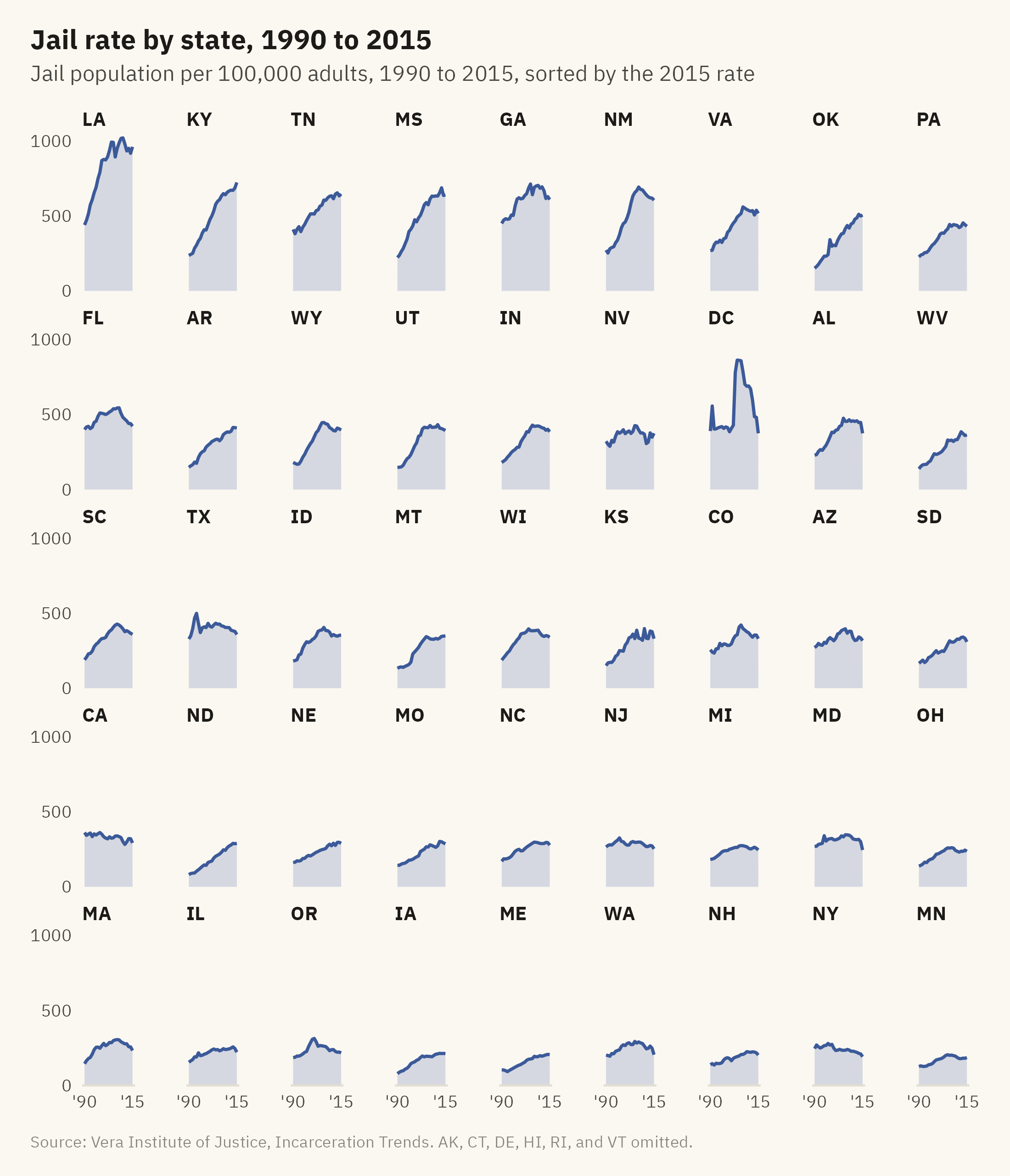
The national line is the sum of fifty state histories. Figure 7.6 shows the jail rate in every state and DC as a grid of small lines, sorted by the 2015 rate.
Show the code
sts <- st |>filter(year >=1990, year <=2015) |>group_by(state) |>filter(all(jail_rate >0)) |>ungroup() |>mutate(state =fct_reorder(state, jail_rate, .fun = \(x) -x[length(x)]))ggplot(sts, aes(year, jail_rate)) +geom_area(fill =mv_accent(), alpha =0.2) +geom_line(color =mv_accent(), linewidth =0.6) +facet_wrap(~ state, ncol =9) +scale_x_continuous(breaks =c(1990, 2015), labels =c("'90", "'15")) +scale_y_continuous(breaks =c(0, 500, 1000), expand =expansion(mult =c(0, 0.05))) +labs(title ="Jail rate by state, 1990 to 2015",subtitle ="Jail population per 100,000 adults, 1990 to 2015, sorted by the 2015 rate",x =NULL, y =NULL, caption =mv_source(src, "AK, CT, DE, HI, RI, and VT omitted")) +theme_mv(base_size =9, grid ="none") +theme(strip.text =element_text(size =rel(0.85), margin =margin(b =1)),axis.text =element_text(size =rel(0.75)), panel.spacing.y =unit(0.5, "lines"),panel.spacing.x =unit(1.4, "lines"))
Figure 7.6: Jail population per 100,000 adults aged 15 to 64 in each state and DC, 1990 to 2015, on a shared vertical scale and sorted by the 2015 rate. Louisiana is far above the rest, at about 960 in 2015. Kentucky, Tennessee, Mississippi, Georgia, and New Mexico form the next group, between 600 and 725. Six states run unified systems with no county jails and are omitted. Source: Vera Institute of Justice, Incarceration Trends.
Forty-five lines on one chart would cross and overlap and could not be followed. Forty-five panels on a shared scale can be read one state at a time. Sorting the panels by the 2015 rate places the highest states first, so a reader can see the ranking without reading the axis of each panel. The shared vertical scale is what allows the comparison across states. With a free scale in each panel, every state’s line would fill its panel, and a reader could not tell a high state from a low one.
7.8 Two Variables Over Time: The Connected Scatter
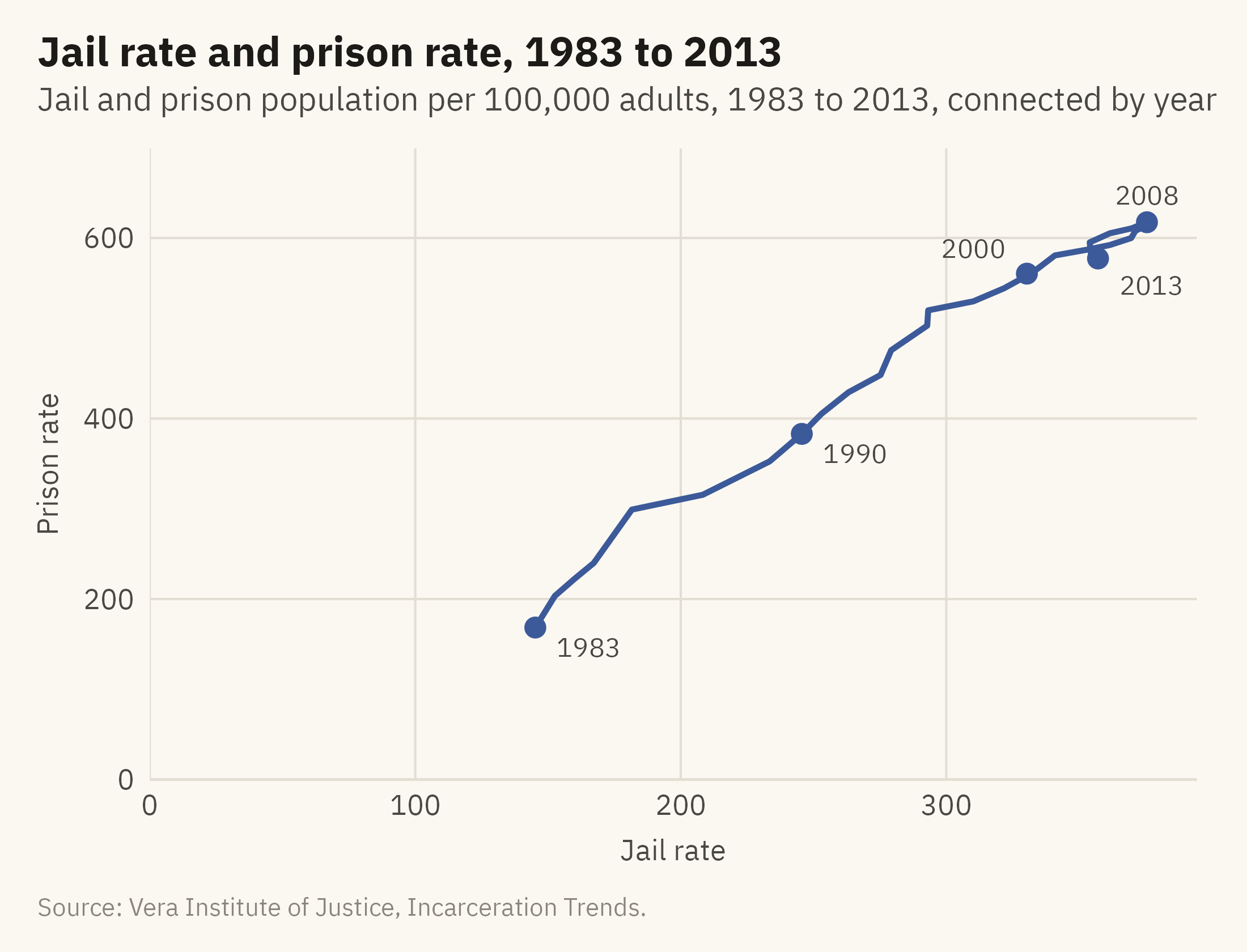
Sometimes the question is how two quantities moved together through time. A connected scatter plot puts one quantity on each axis and draws the path of the years. Figure 7.7 shows the national jail rate against the prison rate from 1983 to 2013.
Show the code
cs <- nat |>filter(year >=1983, year <=2013)marks <- cs |>filter(year %in%c(1983, 1990, 2000, 2008, 2013)) |>mutate(dx =c(8, 8, -8, 0, 8), dy =c(-22, -22, 28, 30, -30), hj =c(0, 0, 1, 0.5, 0))ggplot(cs, aes(jail_rate, prison_rate)) +geom_path(color =mv_accent(), linewidth =0.9, lineend ="round") +geom_point(data = marks, color =mv_accent(), size =2.6) +geom_text(data = marks, aes(x = jail_rate + dx, y = prison_rate + dy, label = year, hjust = hj),size =3, family =mv_font(), color = mv_ink$ink2) +scale_x_continuous(limits =c(0, NA), expand =expansion(mult =c(0, 0.05))) +scale_y_continuous(limits =c(0, NA), expand =expansion(mult =c(0, 0.08))) +labs(title ="Jail rate and prison rate, 1983 to 2013",subtitle ="Jail and prison population per 100,000 adults, 1983 to 2013, connected by year",x ="Jail rate", y ="Prison rate", caption =mv_source(src)) +theme_mv(grid ="y") +theme(panel.grid.major.x =element_line(color = mv_ink$grid, linewidth =0.35))
Figure 7.7: The jail rate against the prison rate, one point per year from 1983 to 2013, connected in order. Both rose together through 2008, when the path turns. From 2008 to 2013 the jail rate fell from 376 to 357 and the prison rate from 617 to 577, so the path doubles back down and to the left along the way it came. Source: Vera Institute of Justice, Incarceration Trends.
Haroz, Kosara, and Franconeri (2016) tested this form against a pair of line charts. They found that readers unfamiliar with the form made more errors, and that a brief explanation of how to read it helped. Label enough years that the reader can follow the direction of the path. Keep the chart to one series. Two paths on one chart tend to cross and become hard to follow.
7.9 Change in a Gap
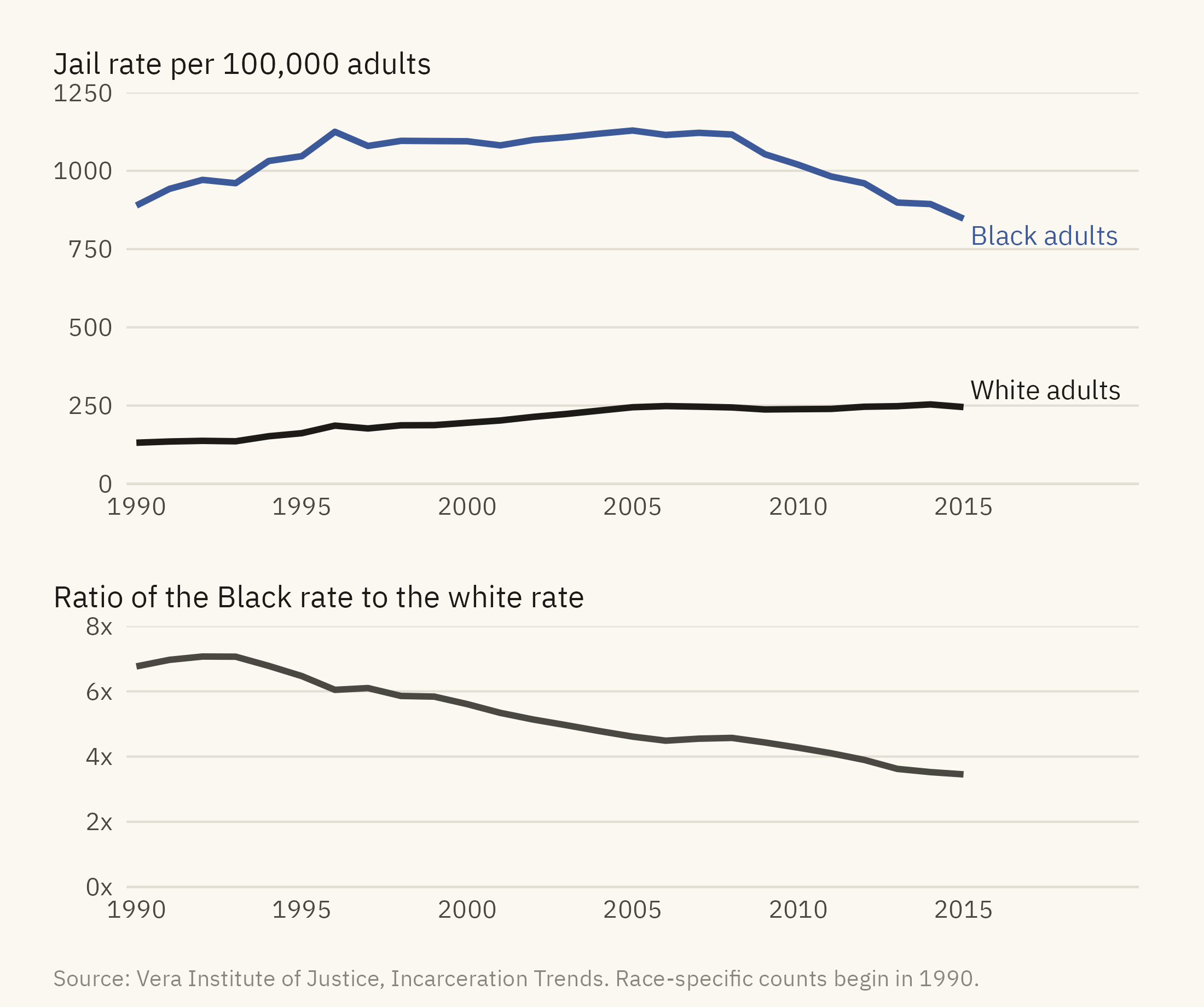
The last question about change is often about a difference between groups. A chart of two lines leaves the reader to estimate the difference between them. Figure 7.8 shows jail rates for Black and white adults and, beneath them, the ratio between the two. The ratio is the quantity being compared, so it is drawn in its own panel.
Show the code
race <- nat |>filter(year >=1990) |>transmute(year, Black =1e5* jail_black / pop_black, White =1e5* jail_white / pop_white, ratio = Black / White)rl <- race |>pivot_longer(c(Black, White), names_to ="group", values_to ="rate")rend <- rl |>filter(year ==2015)p1 <-ggplot(rl, aes(year, rate, color = group)) +geom_line(linewidth =1) +mv_label_end(rend, aes(label =paste(group, "adults"), color = group), nudge_x =0.3) +scale_color_manual(values =c(Black =mv_accent(), White = mv_ink$ink), guide ="none") +scale_x_continuous(breaks =seq(1990, 2015, 5), limits =c(1990, 2020), expand =expansion(mult =0.01)) +scale_y_continuous(limits =c(0, 1250), expand =expansion(0)) +labs(x =NULL, y =NULL, title ="Jail rate per 100,000 adults") +theme_mv(base_size =10) + plain_titlep2 <-ggplot(race, aes(year, ratio)) +geom_line(color = mv_ink$ink2, linewidth =1) +scale_x_continuous(breaks =seq(1990, 2015, 5), limits =c(1990, 2020), expand =expansion(mult =0.01)) +scale_y_continuous(limits =c(0, 8), breaks =c(0, 2, 4, 6, 8), labels = \(x) paste0(x, "x"), expand =expansion(0)) +labs(x =NULL, y =NULL, title ="Ratio of the Black rate to the white rate") +theme_mv(base_size =10) + plain_title(p1 / p2) +plot_layout(heights =c(1.5, 1)) +plot_annotation(caption =mv_source(src, "Race-specific counts begin in 1990"), theme = cap_theme)
Figure 7.8: Jail population per 100,000 adults aged 15 to 64, Black and white, 1990 to 2015 (top), and the ratio between them (bottom). The white rate rose from 131 to about 245 by 2005 and then held there. The Black rate held near 1,100 from 1996 to 2008 and then fell to 847. The ratio fell from near seven to under four. Source: Vera Institute of Justice, Incarceration Trends. Race-specific counts begin in 1990.
When the question is about the gap between two series, draw the gap directly. Three ways to do so are a panel showing the ratio of the two series, a panel showing their difference, or a shaded band between the two lines. With the two lines alone, a reader has to estimate the vertical distance between two positions that do not share a baseline. Cleveland and McGill (1984), described in Chapter 2, found that readers judge such comparisons less accurately than positions on a common scale.
ImportantEthics Moment: A Snapshot Is Not a Year
Every number in this chapter counts people on one day. A jail that holds 100 people on December 31 may have held 2,000 different people over the year, most of them for a few days. The surveys measure the one-day count, and every chart in this chapter shows that count. Because most jail stays are short, a one-day count includes only a small share of the people who passed through jail that year. Sawyer and Wagner (2023) report several million jail admissions per year in the United States against a one-day count of several hundred thousand. The caption of a chart over time should state what was counted and when. “People in jail” and “people who went to jail” are different quantities, and the difference between them is millions of people.
TipTry It Online
Time and Base at viz.marginoferrormedia.com/apps holds the state-by-year data. Pick any set of states, switch between counts, rates, and an index, and move the base year with a slider. Notice how the choice of base year changes which states appear to be growing. A coverage bar under the chart shows how many counties reported in each year.
WarningAI Reality Check: The Line Through the Gap
A model asked to chart the prison population from this file will usually sum the counties and draw a line that falls by a fifth after 2013. It will then often describe a sharp decline in incarceration, and it may offer reasons for it. The chart is an accurate sum of the rows in the file. The sentence about a decline is wrong, because the rows are incomplete after 2013. The model does not usually check coverage unless the prompt asks for it. A line drawn from a series with incomplete coverage looks the same as a line drawn from a complete one.
For every series, ask how many units reported in each year and whether the definition changed. A model can often answer that question well when asked. It rarely asks the question on its own.
7.10 Putting It All Together
A line chart is the usual form for change over time. When the reader is expected to compare sizes, the vertical axis starts at zero. A count should be checked against its rate, because growth in the base can account for part of a rise. Two series of similar size can be placed on one scale with direct labels. Series of different sizes can be indexed to a base year, with the base year stated on the chart. Many places can be shown as small multiples on a shared scale. The joint movement of two variables can be shown as a connected scatter plot. When a gap between groups is the main point, the gap needs its own panel or band. Before any of this, the number of units reporting in each period should be checked, and the series should end where full coverage ends.
7.11 Looking Ahead
Chapter 8 covers the question of where, which is answered with a map. Maps have problems of their own. A reader tends to see land area as if it were population, counts are often mapped where rates are needed, and color intensity is judged less accurately than position or length. The case is housing cost and water access by county, where the pattern on the map differs from the pattern in the population.
7.12 Further Reading and References
Cleveland, W. S. (1994). The Elements of Graphing Data, 2nd edition. Hobart Press. On banking to 45 degrees and the aspect ratio of time series.
Haegeli, A., and Vera Institute of Justice (2018). Incarceration Trends: Data and Methods. The documentation for the dataset, including the coverage notes behind Figure 7.5.
Haneman, M. (2015). Connected scatterplots. The Functional Art, and Haroz, S., Kosara, R., and Franconeri, S. (2016). The connected scatterplot for presenting paired time series. IEEE Transactions on Visualization and Computer Graphics, 22(9), 2174–2186. Evidence on when the connected scatter helps and when it confuses.
Sawyer, W., and Wagner, P. (2023). Mass Incarceration: The Whole Pie. Prison Policy Initiative. The standard annual summary of who is held where, with a clear account of snapshot versus admission counts.
Tufte, E. R. (2001). The Visual Display of Quantitative Information, 2nd edition. Graphics Press. The time series chapter, and the discussion of the lie factor applied to time axes.
7.13 Key Terms
Line chart. One quantity connected across time. The connection lets a reader see the series as one object rather than as separate points.
Rate. A count divided by its base. It separates growth in the thing measured from growth in the base.
Index chart. Each series divided by its value in a base year, so that slopes show growth rates. It leaves out the levels.
Coverage. How many units reported in each period. A series is reliable only for the periods in which coverage is complete.
Small multiples over time. One panel per place on a shared scale, sorted so that the order of the panels shows a ranking.
Connected scatter plot. Two variables on the axes, with the years joined as a path.
Snapshot count. The number of people in a state on one day, as distinct from the number who passed through it over a period.
7.14 Exercises
Check Your Understanding
Figure 7.1 starts its axis at zero. Give the reason, and describe a version of the chart where starting at 100,000 would be defensible.
The jail count and jail rate have the same shape in Figure 7.2. What would it mean if the rate had been flat while the count rose?
Why does the index chart in Figure 7.4 make the prison line look steeper than Figure 7.3 does? What does it leave out?
Describe the problem in Figure 7.5 in one sentence a manager could act on.
In Figure 7.7, what does a horizontal stretch of the path mean? A vertical one?
Apply It
Using ch07-incarceration-state.csv, draw the jail rate for your state against the national rate on one chart from zero, with direct labels. Write the title as a finding.
Re-index Figure 7.4 to 2008 instead of 1983 and describe how the picture changes. Which base year is the fairer choice, and why?
Draw the small multiples in Figure 7.6 with free vertical scales. Pick one state whose pattern looks different and explain what the free scale did to it.
Compute the ratio of the Black jail rate to the white rate for each state in 2015 and draw it as a dot plot. Which states are furthest from the national ratio?
Think Deeper
The chapter cuts the prison series at 2013. Propose a method for estimating the 2014 and 2015 totals from the counties that did report, and say what a chart of that estimate would need to disclose.
The Ethics Moment distinguishes people in jail from people who went to jail. Which quantity should a chart about the reach of the jail system show, and what data would it need?
A news chart shows incarceration “down 21 percent since 2013” using this data. Write a short letter to the editor that explains the error without accusing anyone of bad faith.