4  Comparison and Composition

4.1 Where People Go When They Flee

At the end of 2022, UNHCR counted 29 million refugees. These are people who have left their own country to escape persecution, war, or violence. A count of 29 million is hard to interpret on its own. Four narrower questions can be asked of it. Where did these people come from, where did they go, how far did they go, and has that changed over time. Each of those questions is a comparison or a composition. This chapter covers the chart forms that answer them.

Comparison is the question of how one value compares with others. For example, how many refugees came from Syria compared with Afghanistan or Ukraine. Composition is the question of how a whole divides into parts. For example, of the refugees from Syria, what share is in Türkiye, what share is in Germany, and what share is everywhere else. The two questions call for different chart forms. A common error is to answer a comparison question with a composition chart, or the reverse.

4.2 The Bar Chart, Done Properly

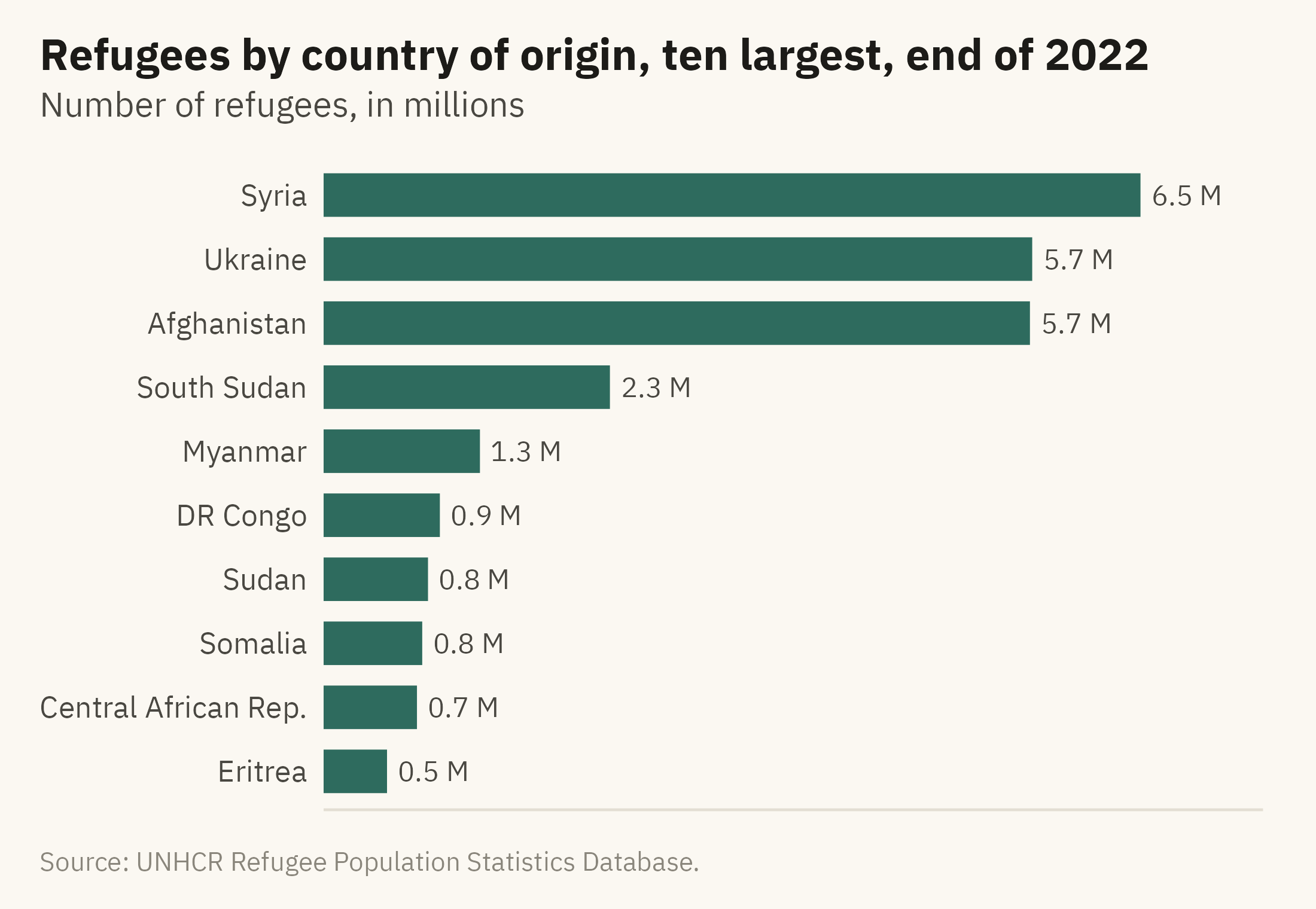
The bar chart is the most common form for comparing values across categories. Four rules address most of the errors that appear in bar charts. Figure 4.1 shows the ten largest countries of origin in 2022, drawn by those rules.

orig22 <- w |> filter(year == 2022) |> group_by(origin) |> summarise(r = sum(refugees), .groups = "drop")
top10 <- orig22 |> slice_max(r, n = 10) |> mutate(origin = fct_reorder(origin, r))
share3 <- sum(head(arrange(orig22, -r), 3)$r) / sum(orig22$r)

ggplot(top10, aes(r, origin)) +
  geom_col(fill = mv_accent(), width = 0.68) +
  geom_text(aes(label = label_comma(scale = 1e-6, accuracy = 0.1, suffix = " M")(r)),
            hjust = -0.15, size = 3, family = mv_font(), color = mv_ink$ink2) +
  scale_x_continuous(expand = expansion(mult = c(0, 0.15))) +
  labs(title = "Refugees by country of origin, ten largest, end of 2022",
       subtitle = "Number of refugees, in millions",
       x = NULL, y = NULL, caption = mv_source(src)) +
  theme_mv(grid = "none") +
  theme(axis.text.x = element_blank())

Figure 4.1: Refugees by country of origin at the end of 2022, ten largest. Three countries account for about three-fifths of the world’s refugees. Source: UNHCR Refugee Population Statistics Database.

Sort the bars by value unless the categories have a natural order, such as months or age groups. In a sorted chart, the reader can find the largest and smallest values without searching. Run them horizontally when the labels are words. Country names fit beside horizontal bars. Under vertical bars, labels of that length overlap or have to be rotated. Start at zero, because a bar encodes its value as length, as Chapter 2 explained. Label the values when the reader will want them, and drop the axis once the labels make it redundant. Figure 4.1 has no horizontal axis because each bar has its value printed beside it.

A further decision is how many bars to show. The data include about 200 countries and territories of origin, and Figure 4.1 shows ten. A chart of all of them would need several pages, and most of the bars would be too short to compare. The title says “ten largest” so the reader knows what was left out. The caption gives the share of the three largest.

4.3 Comparing Two Moments

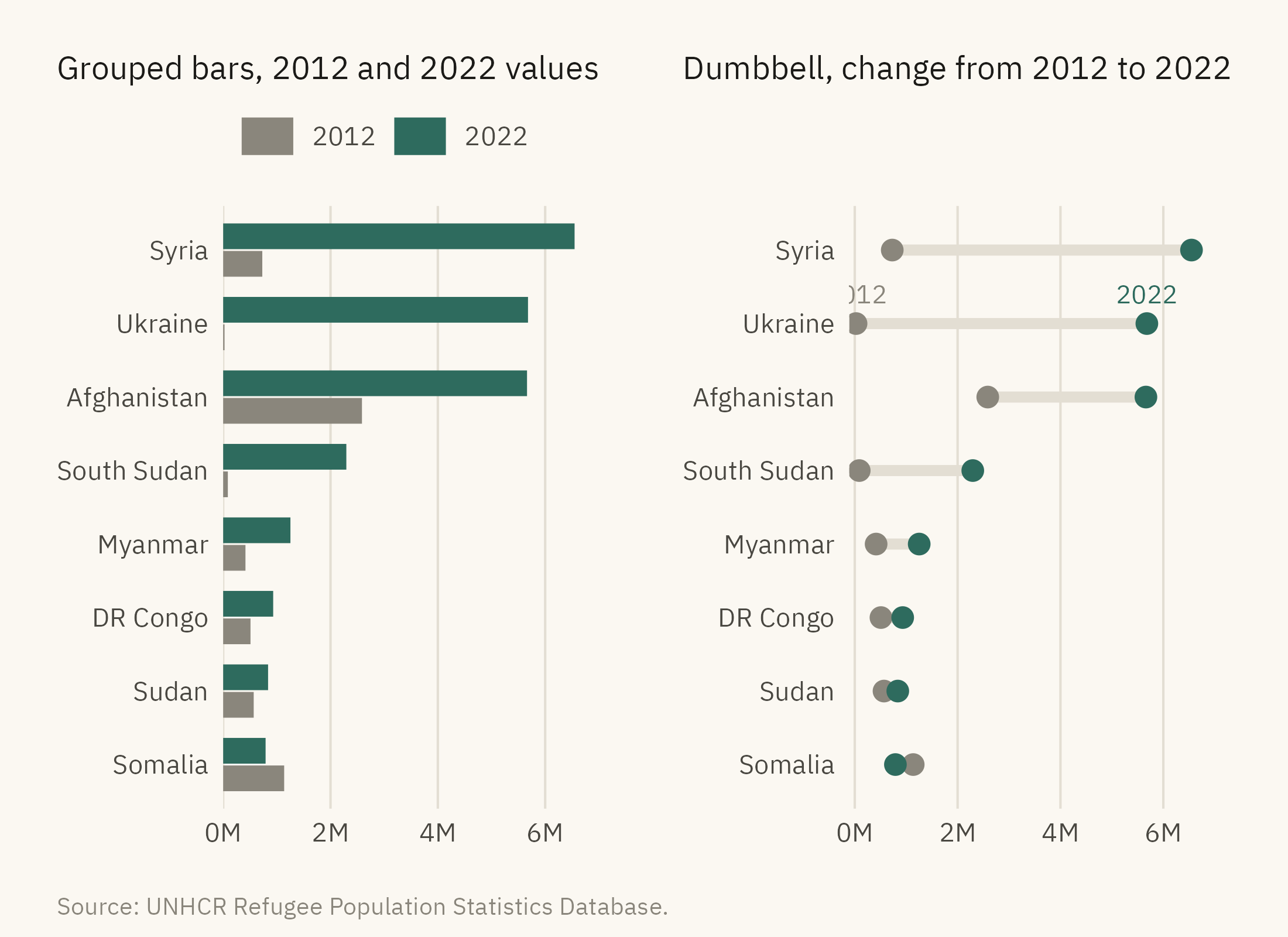
A comparison of two points in time is a common request in business reports, such as revenue this year against last year by region. Here the comparison is refugees in 2022 against 2012, by country of origin. The usual first choice is a grouped bar chart, with two bars per category. Figure 4.2 shows a grouped bar chart on the left and a dumbbell chart on the right.

two <- w |> filter(year %in% c(2012, 2022)) |> group_by(origin, year) |> summarise(r = sum(refugees), .groups = "drop") |>
  pivot_wider(names_from = year, values_from = r, names_prefix = "y", values_fill = 0) |>
  slice_max(y2022, n = 8) |> mutate(origin = fct_reorder(origin, y2022))

grouped <- two |> pivot_longer(c(y2012, y2022), names_to = "year", values_to = "r") |>
  mutate(year = str_remove(year, "y")) |>
  ggplot(aes(r, origin, fill = year)) +
  geom_col(position = position_dodge(width = 0.75), width = 0.7) +
  scale_fill_manual(values = c(`2012` = mv_ink$mute, `2022` = mv_accent()), name = NULL) +
  scale_x_continuous(labels = label_comma(scale = 1e-6, suffix = "M"), expand = expansion(mult = c(0, 0.05))) +
  labs(x = NULL, y = NULL, title = "Grouped bars, 2012 and 2022 values") +
  theme_mv(base_size = 10, grid = "x") + plain_title

dumbbell <- ggplot(two) +
  geom_segment(aes(x = y2012, xend = y2022, y = origin, yend = origin), color = mv_ink$grid, linewidth = 1.6) +
  geom_point(aes(y2012, origin), color = mv_ink$mute, size = 2.6) +
  geom_point(aes(y2022, origin), color = mv_accent(), size = 2.6) +
  annotate("text", x = two$y2012[two$origin == "Ukraine"], y = "Ukraine", label = "2012", vjust = -1.1,
           size = 2.8, family = mv_font(), color = mv_ink$mute) +
  annotate("text", x = two$y2022[two$origin == "Ukraine"], y = "Ukraine", label = "2022", vjust = -1.1,
           size = 2.8, family = mv_font(), color = mv_accent()) +
  scale_x_continuous(labels = label_comma(scale = 1e-6, suffix = "M"), expand = expansion(mult = c(0.02, 0.08))) +
  labs(x = NULL, y = NULL, title = "Dumbbell, change from 2012 to 2022") +
  theme_mv(base_size = 10, grid = "x") + plain_title

grouped + dumbbell + plot_annotation(caption = mv_source(src), theme = cap_theme)

Figure 4.2: Refugees by country of origin in 2012 and 2022 for the eight largest in 2022. Left, grouped bars. The reader compares pairs of lengths. Right, a dumbbell chart. The change is drawn as a line, so the reader can compare changes across countries. Ukraine and South Sudan had few refugees in 2012. Source: UNHCR Refugee Population Statistics Database.

In a dumbbell chart, the length of the connecting line is the change. The reader compares eight lengths rather than sixteen. The accent color marks the 2022 end, so the direction of change can be seen. Ukraine’s 2012 value is close to zero, so its line runs almost the full distance to its 2022 value. In the grouped bars, the same change has to be found by comparing a very short bar with a long one. When the question is about change rather than levels, the dumbbell encodes the change directly as a length.

With more than about twelve categories, both forms become crowded. The slope chart from Chapter 1 and the dot plot later in this chapter can show more categories.

4.4 Composition: The Stacked Bar

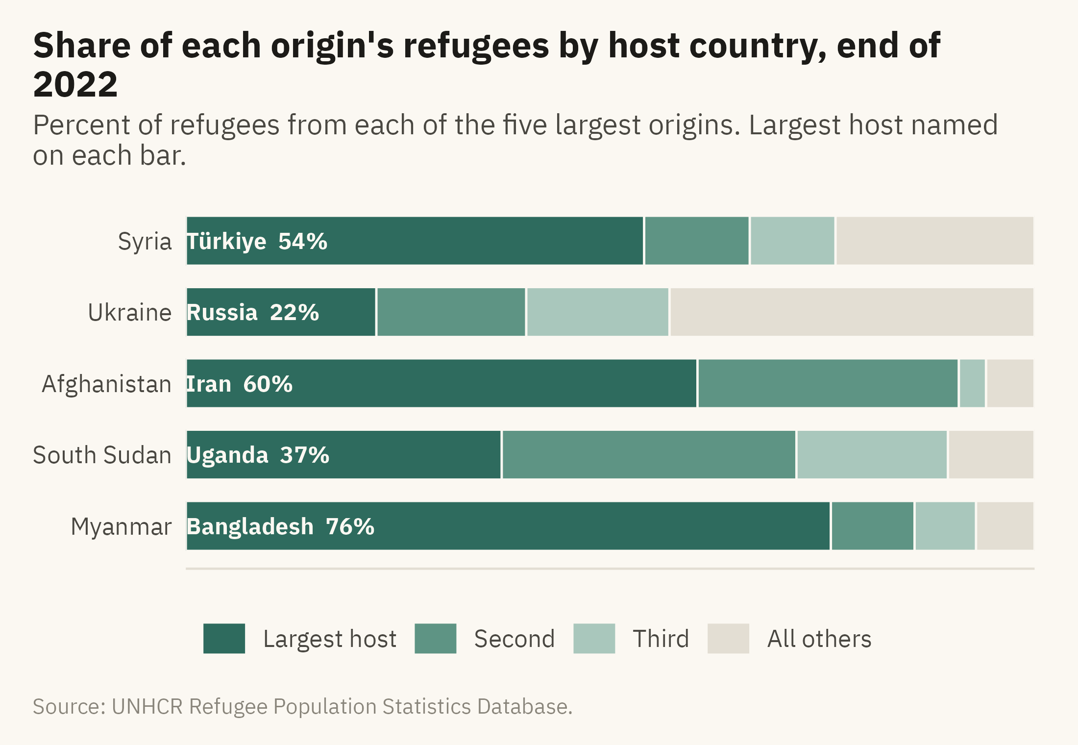
Chapter 3 showed a stacked area chart in which the middle layers could not be compared. In any stacked chart, every layer above the first starts at a different height, so the reader has to compare positions on scales that do not line up. Chapter 2 placed that comparison below length on the hierarchy. Stacking is suitable when the total is the main point and the parts are few. Figure 4.3 shows where the refugees from each of the five largest origin countries were hosted. For four of the five, the largest host was a neighboring country.

five <- head(arrange(orig22, -r), 5)$origin
comp <- w |> filter(year == 2022, origin %in% five) |>
  group_by(origin, asylum) |> summarise(r = sum(refugees), .groups = "drop") |>
  group_by(origin) |> arrange(-r, .by_group = TRUE) |>
  mutate(rank = row_number(), host = case_when(rank == 1 ~ asylum, rank == 2 ~ asylum, rank == 3 ~ asylum, TRUE ~ "All others"),
         slot = case_when(rank == 1 ~ "Largest host", rank == 2 ~ "Second", rank == 3 ~ "Third", TRUE ~ "All others")) |>
  group_by(origin, slot, host) |> summarise(r = sum(r), .groups = "drop") |>
  group_by(origin) |> mutate(share = r / sum(r), total = sum(r)) |> ungroup() |>
  mutate(slot = factor(slot, levels = rev(c("Largest host", "Second", "Third", "All others"))),
         origin = fct_reorder(origin, total),
         label = if_else(slot == "Largest host", paste0(host, "  ", percent(share, 1)), ""))

ggplot(comp, aes(share, origin, fill = slot)) +
  geom_col(width = 0.7, color = mv_ink$canvas, linewidth = 0.4) +
  geom_text(aes(label = label, x = 0.01), position = position_stack(vjust = 0, reverse = FALSE),
            hjust = 0, size = 3, family = mv_font(), color = mv_ink$canvas, fontface = "bold") +
  scale_fill_manual(values = c(`Largest host` = mv_accent(), Second = "#5E9484", Third = "#A9C7BC", `All others` = mv_ink$grid),
                    breaks = c("Largest host", "Second", "Third", "All others"), name = NULL) +
  scale_x_continuous(labels = label_percent(), expand = expansion(0)) +
  labs(title = "Share of each origin's refugees by host country, end of 2022",
       subtitle = "Percent of refugees from each of the five largest origins. Largest host named on each bar.",
       x = NULL, y = NULL, caption = mv_source(src)) +
  theme_mv(grid = "none") +
  theme(legend.position = "bottom", axis.text.x = element_blank())

Figure 4.3: Where the refugees from the five largest countries of origin were hosted at the end of 2022, as shares. In each row the darkest segment is the single largest host country, named on the bar. For four of the five, the largest host was a neighboring country. Source: UNHCR Refugee Population Statistics Database.

Figure 4.3 differs from the stacked area in Chapter 3 in three ways. First, the bars sum to 100 percent, so the reader can read any segment as a share of the whole. Secondly, there are four segments rather than eight. Thirdly, the segments appear in the same order in every bar, largest first, so the first segment can be compared across rows by its length from the left edge. Türkiye hosts 54 percent of refugees from Syria. Uganda hosts 37 percent of those from South Sudan. Iran hosts 60 percent of those from Afghanistan. Ukraine is the exception, because its refugees are spread across many European countries. In the chart, Ukraine’s row has a short first segment and a long grey segment at the right.

A 100 percent stacked bar is suitable when the question is “what share” and the parts are few. When the question is “how many,” use the counts and let the bars differ in length. Showing both on one chart is not advised, because the reader then has to judge both the length of each bar and the division within it.

4.5 The Pie, in Its One Good Use

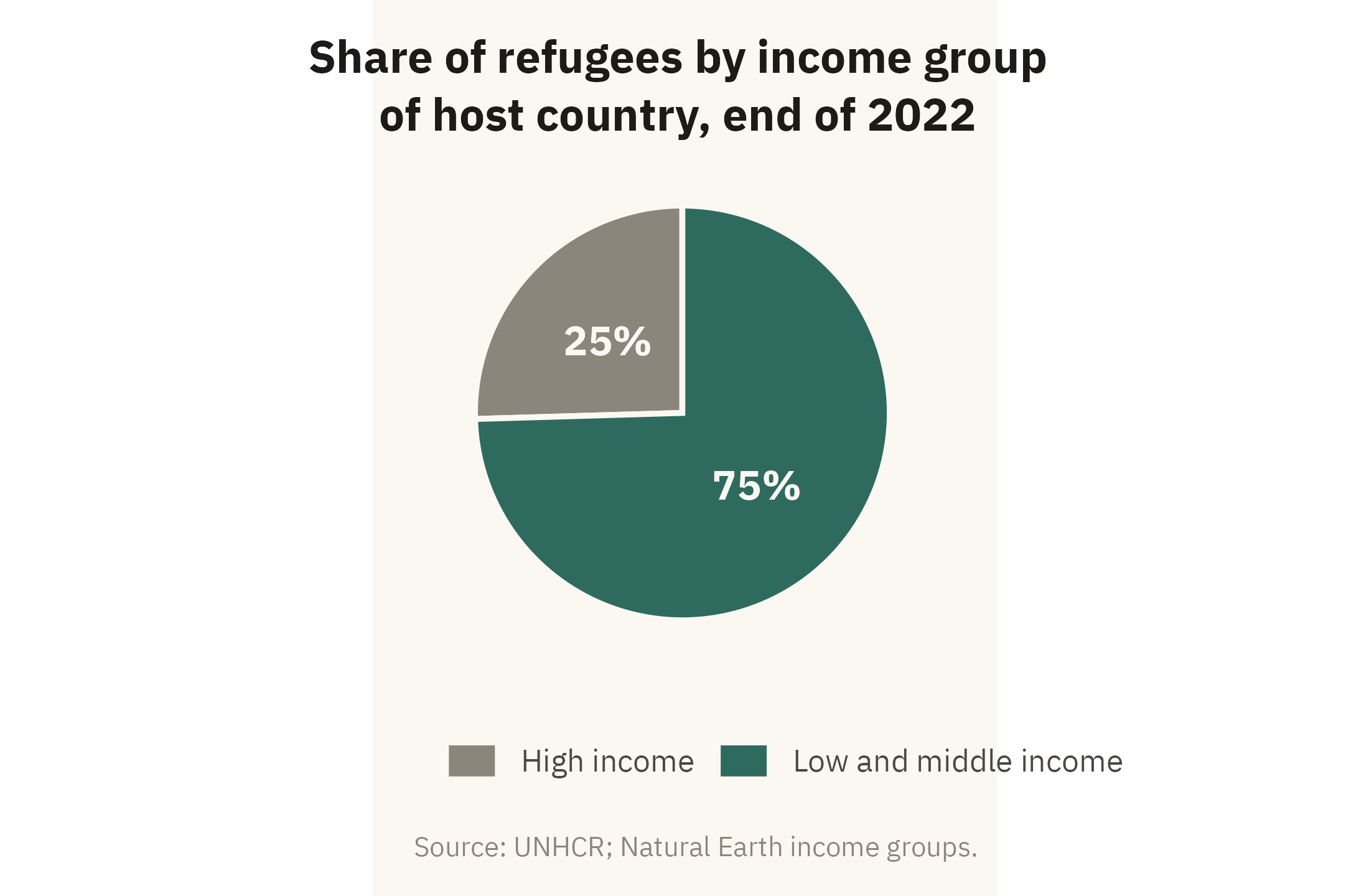
A pie chart is suitable for one question. With two or three slices, a reader can judge whether a share is near a half, a third, or a quarter. Chapter 2 made the same point for a slice that is about half of the whole. Figure 4.4 uses a pie for that purpose only.

inc <- w |> filter(year == 2022, !is.na(asylum_income)) |>
  mutate(grp = if_else(asylum_income == "High income", "High income", "Low and middle income")) |>
  group_by(grp) |> summarise(r = sum(refugees), .groups = "drop") |> mutate(share = r / sum(r))

ggplot(inc, aes(x = 1, y = share, fill = grp)) +
  geom_col(width = 1, color = mv_ink$canvas, linewidth = 0.8) +
  coord_polar(theta = "y", start = 0) +
  geom_text(aes(label = percent(share, 1)), position = position_stack(vjust = 0.5), size = 4.2,
            family = mv_font(), color = mv_ink$canvas, fontface = "bold") +
  scale_fill_manual(values = c(`High income` = mv_ink$mute, `Low and middle income` = mv_accent()), name = NULL) +
  labs(title = "Share of refugees by income group\nof host country, end of 2022",
       caption = mv_source("UNHCR; Natural Earth income groups")) +
  theme_mv_blank() + theme(legend.position = "bottom", plot.title = element_text(hjust = 0.5, lineheight = 1.05))

Figure 4.4: Share of the world’s refugees hosted by countries in each World Bank income group, end of 2022. Three in four are in low- and middle-income countries. A pie is suitable here because the reader only needs to see that the high-income slice is about a quarter. Source: UNHCR; income groups from Natural Earth.

The chart has two slices with one number printed on each, so the reader does not need to compare angles. When a third category matters, or when the reader needs to tell 25 percent from 21 percent, the reader has to compare angles. Cleveland and McGill (1984) found those judgments less accurate than comparisons of length. A bar chart is the more accurate choice in both cases.

4.6 Many Categories: The Dot Plot

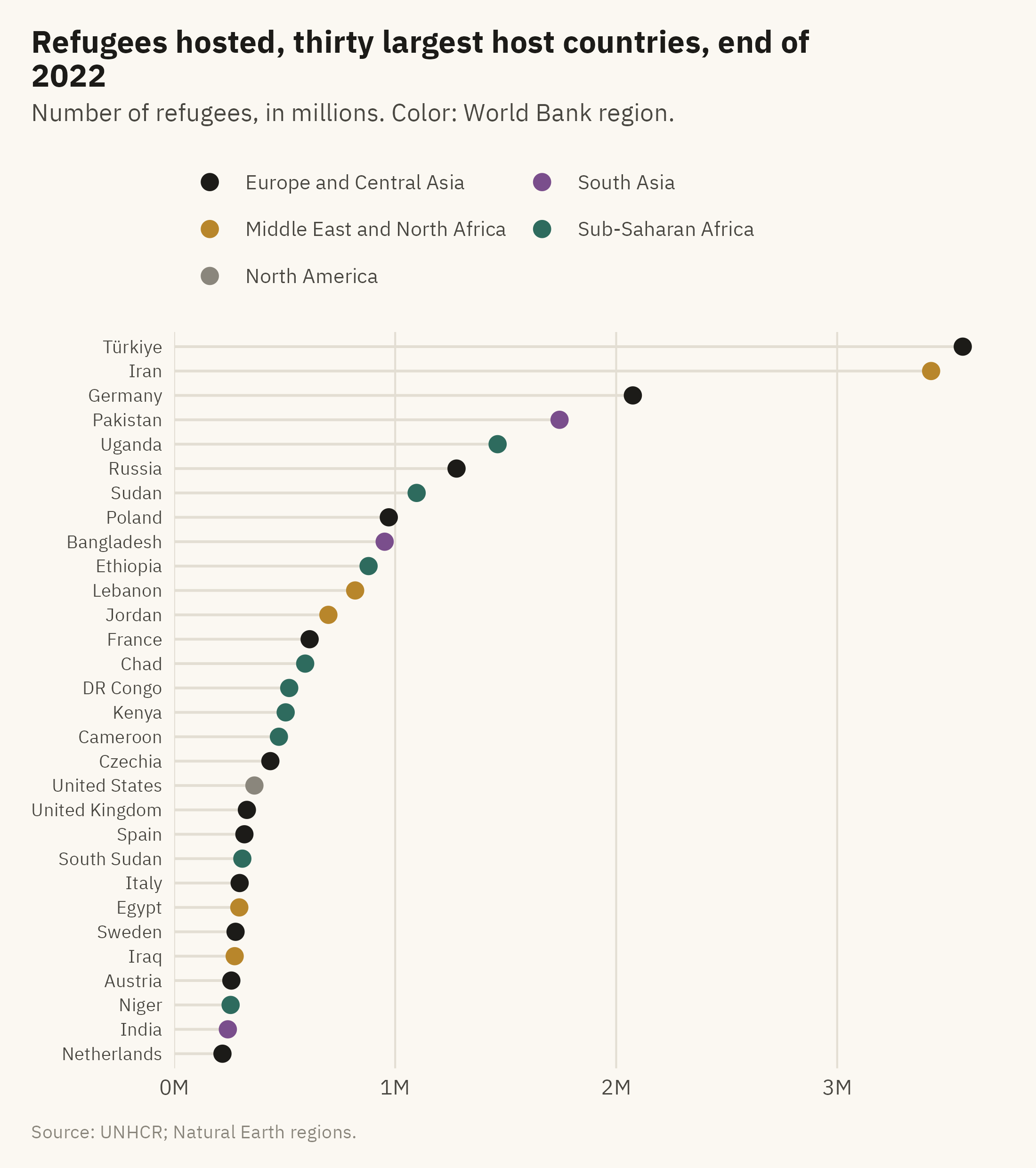
With forty categories, bars become thin and the chart becomes tall. A dot plot, described by Cleveland (1994), shows the same values as points on a common scale. The hierarchy in Chapter 2 ranks position on a common scale as the most accurate encoding. A dot plot also uses less ink than a bar chart, so forty rows can fit on a page. Figure 4.5 shows the thirty largest host countries, with color for region.

hosts30 <- w |> filter(year == 2022, !is.na(asylum_region)) |>
  group_by(asylum, asylum_region) |> summarise(r = sum(refugees), .groups = "drop") |>
  slice_max(r, n = 30) |>
  mutate(asylum = fct_reorder(asylum, r),
         asylum_region = str_replace(asylum_region, " & ", " and "))
reg_cols <- c("Sub-Saharan Africa" = mv_accent(), "Middle East and North Africa" = "#B8862B",
              "Europe and Central Asia" = "#1C1B18", "South Asia" = "#7A4E8C",
              "East Asia and Pacific" = "#5B6E8C", "Latin America and Caribbean" = "#C25B2A",
              "North America" = "#8A867C")
ggplot(hosts30, aes(r, asylum, color = asylum_region)) +
  geom_segment(aes(x = 0, xend = r, yend = asylum), color = mv_ink$grid, linewidth = 0.5) +
  geom_point(size = 2.6) +
  scale_color_manual(values = reg_cols, name = NULL) +
  scale_x_continuous(labels = label_comma(scale = 1e-6, suffix = "M"), expand = expansion(mult = c(0, 0.04))) +
  guides(color = guide_legend(ncol = 2)) +
  labs(title = "Refugees hosted, thirty largest host countries, end of 2022",
       subtitle = "Number of refugees, in millions. Color: World Bank region.",
       x = NULL, y = NULL, caption = mv_source("UNHCR; Natural Earth regions")) +
  theme_mv(base_size = 10, grid = "x") +
  theme(legend.text = element_text(size = rel(0.78)), axis.text.y = element_text(size = rel(0.85)))

Figure 4.5: The thirty countries hosting the most refugees at the end of 2022. Position encodes the count. Color groups the countries by World Bank region. Source: UNHCR; regions from Natural Earth.

The thin grey lines are optional. On a wide chart they help the reader follow a row from the label to the dot, and they add only thin lines. Without them the chart is a plain dot plot. With them it is sometimes called a lollipop chart. In both versions the dots encode the data. The chart fits thirty categories in the space where bars of readable width would fit about fifteen.

4.7 Many Parts: The Treemap

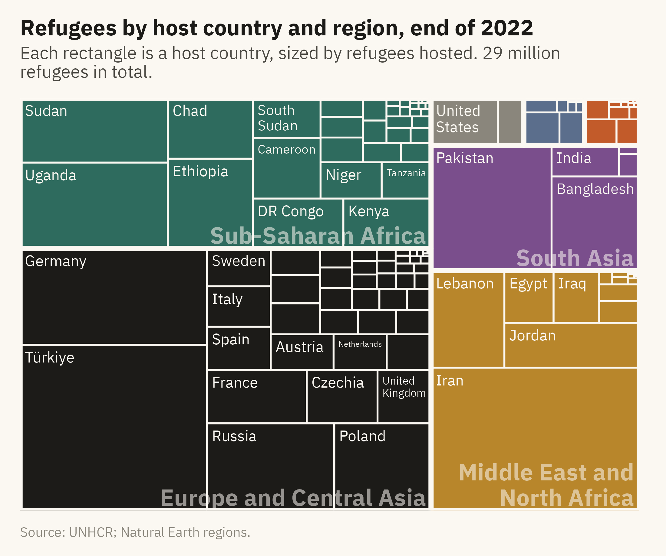
Some compositions have dozens of parts at two levels, such as host region and host country. A treemap, introduced by Shneiderman (1992), shows them as nested rectangles sized by value. Area is low on the hierarchy from Chapter 2, so a reader cannot compare two rectangles with precision. A treemap is suited to questions about how a whole is divided. A reader can see which region hosts the most refugees, which countries within that region host the most, and how many small hosts there are. Figure 4.6 shows all 29 million refugees by host country and region.

tm <- w |> filter(year == 2022, !is.na(asylum_region)) |>
  group_by(asylum_region, asylum) |> summarise(r = sum(refugees), .groups = "drop") |>
  mutate(asylum_region = str_replace(asylum_region, " & ", " and "),
         lab = if_else(r >= 200000, asylum, ""),
         # Small regions get a blank subgroup name so no label is drawn over their tiles.
         # Distinct whitespace strings keep each region as its own subgroup in the layout.
         region_lab = case_when(asylum_region == "North America" ~ " ",
                                asylum_region == "East Asia and Pacific" ~ "  ",
                                asylum_region == "Latin America and Caribbean" ~ "   ",
                                TRUE ~ asylum_region))
ggplot(tm, aes(area = r, fill = asylum_region, subgroup = region_lab, label = lab)) +
  geom_treemap(color = mv_ink$canvas, size = 1.5) +
  geom_treemap_subgroup_border(color = mv_ink$canvas, size = 4) +
  geom_treemap_text(color = mv_ink$canvas, family = mv_font(), size = 9, min.size = 4,
                    padding.x = grid::unit(1, "mm"), padding.y = grid::unit(1.5, "mm"), reflow = TRUE) +
  geom_treemap_subgroup_text(color = mv_ink$canvas, family = mv_font(), fontface = "bold", alpha = 0.55,
                             size = 14, place = "bottomright", grow = FALSE, reflow = TRUE) +
  scale_fill_manual(values = reg_cols, guide = "none") +
  labs(title = "Refugees by host country and region, end of 2022",
       subtitle = "Each rectangle is a host country, sized by refugees hosted. 29 million refugees in total.",
       caption = mv_source("UNHCR; Natural Earth regions")) +
  theme_mv_blank()

Figure 4.6: All refugees at the end of 2022 by host region and host country. Each rectangle is a host country, sized by the number of refugees and grouped by region. Countries hosting fewer than 200,000 are unlabeled. The three smallest regions, North America, East Asia and Pacific, and Latin America and Caribbean, are too small to name on the chart. Source: UNHCR; regions from Natural Earth.

Use a treemap to show how a whole with many parts is divided. Do not use it to compare any two parts. If the finding is “Türkiye hosts more refugees than Iran,” draw bars. If the finding is “most refugees are in a small number of countries across three regions,” draw the treemap.

4.8 Comparing Within and Across Groups

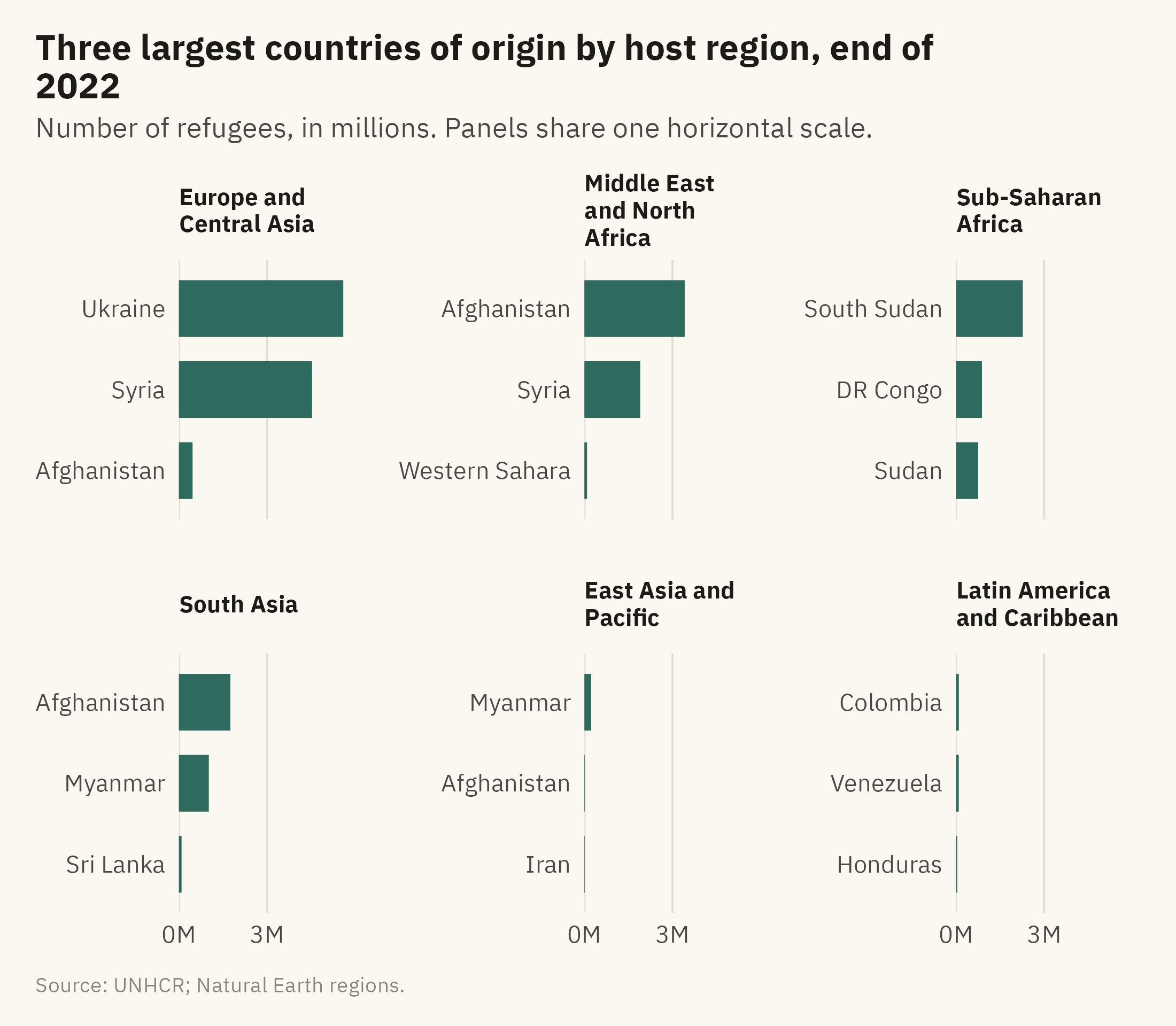
The last form in this chapter is for a two-level comparison. The question here is which origins are largest in each host region. One chart with region on one axis and origin on the other is a heatmap, which Chapter 9 covers. For a few groups, small multiples of bars are simpler. There is one panel per region, and each panel is sorted on its own. Figure 4.7 shows the three largest origins for each of six host regions.

by_reg <- w |> filter(year == 2022, !is.na(asylum_region), asylum_region != "North America") |>
  group_by(asylum_region, origin) |> summarise(r = sum(refugees), .groups = "drop") |>
  group_by(asylum_region) |> slice_max(r, n = 3) |> ungroup() |>
  mutate(asylum_region = str_replace(asylum_region, " & ", " and "),
         asylum_region = str_wrap(asylum_region, 14),
         asylum_region = fct_reorder(asylum_region, r, .fun = max, .desc = TRUE),
         origin = paste0(origin, "___", as.integer(asylum_region)))
by_reg <- by_reg |> mutate(origin = fct_reorder(origin, r))
ggplot(by_reg, aes(r, origin)) +
  geom_col(fill = mv_accent(), width = 0.7) +
  facet_wrap(~ asylum_region, ncol = 3, scales = "free_y") +
  scale_y_discrete(labels = \(x) str_remove(x, "___\\d+$")) +
  scale_x_continuous(labels = label_comma(scale = 1e-6, suffix = "M"), breaks = c(0, 3e6, 6e6),
                     expand = expansion(mult = c(0, 0.05))) +
  labs(title = "Three largest countries of origin by host region, end of 2022",
       subtitle = "Number of refugees, in millions. Panels share one horizontal scale.",
       x = NULL, y = NULL, caption = mv_source("UNHCR; Natural Earth regions")) +
  theme_mv(base_size = 10, grid = "x") +
  theme(strip.text = element_text(size = rel(0.8), lineheight = 0.95))

Figure 4.7: The three largest countries of origin for refugees hosted in each World Bank region, end of 2022. Each panel is sorted on its own, and the panels share one horizontal scale so sizes can be compared across regions. Source: UNHCR; regions from Natural Earth.

The shared horizontal scale is a design choice. With it, the bars for Sub-Saharan Africa are short next to those for the Middle East and Europe, which reflects the counts. With a free scale in each panel, every panel would fill its frame, and the reader could not compare sizes across regions. The choice of scale depends on which comparison the reader needs, within panels or across them.

4.9 Flows and Connections

The charts so far compare amounts in one place or at one time. Two other questions arise with the same data. Where do people go, from which country to which? And which countries are connected to each other by those movements? The first is a question about flows, and the second is a question about a network.

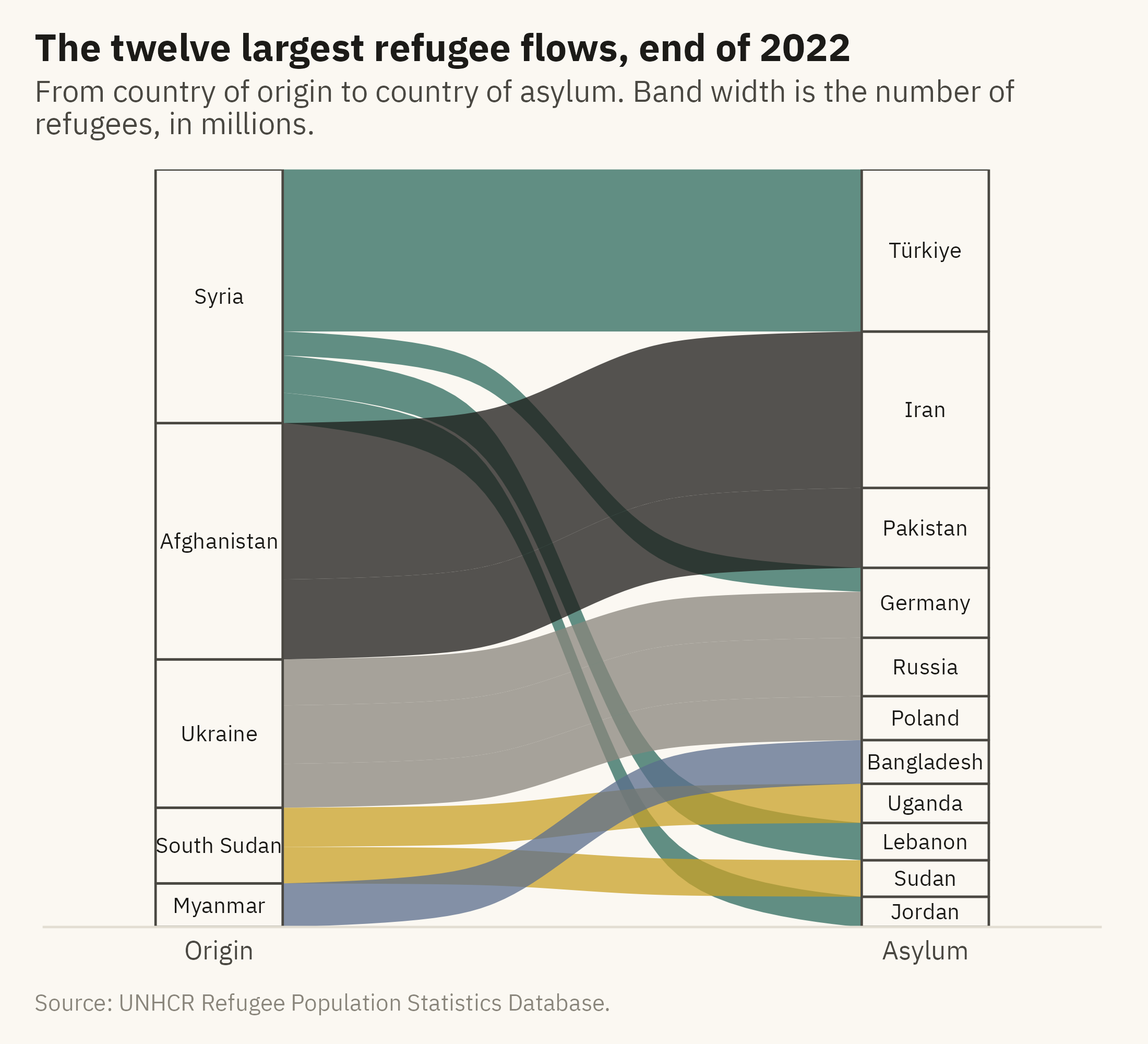
A Sankey diagram shows flows. It draws each origin and each destination as a block, and a band between them whose width is proportional to the number of people who moved. Figure 4.8 shows the twelve largest refugee flows at the end of 2022, which together hold about 56 percent of the world’s refugees. The width of each band can be compared by eye, since width is a length. The diagram also shows structure that a bar chart would not. Syria’s refugees are in four countries. Ukraine’s are in three. Afghanistan’s are almost all in two neighbors.

flows <- w |> filter(year == 2022) |>
  group_by(origin, asylum) |> summarise(n = sum(refugees), .groups = "drop") |>
  slice_max(n, n = 12) |>
  mutate(origin = fct_reorder(origin, n, .fun = sum, .desc = TRUE),
         asylum = fct_reorder(asylum, n, .fun = sum, .desc = TRUE))
ggplot(flows, aes(axis1 = origin, axis2 = asylum, y = n)) +
  geom_alluvium(aes(fill = origin), width = 0.18, alpha = 0.75, knot.pos = 0.4) +
  geom_stratum(width = 0.18, fill = mv_ink$canvas, color = mv_ink$ink2, linewidth = 0.4) +
  geom_text(stat = "stratum", aes(label = after_stat(stratum)), size = 2.7, family = mv_font(), color = mv_ink$ink) +
  scale_x_discrete(limits = c("Origin", "Asylum"), expand = expansion(mult = 0.25)) +
  scale_fill_manual(values = mv_series(6), guide = "none") +
  scale_y_continuous(labels = label_comma(scale = 1e-6, suffix = "M"), expand = expansion(0)) +
  labs(title = "The twelve largest refugee flows, end of 2022",
       subtitle = "From country of origin to country of asylum. Band width is the number of refugees, in millions.",
       x = NULL, y = NULL, caption = mv_source(src)) +
  theme_mv(grid = "none") + theme(axis.text.y = element_blank())

Figure 4.8: The twelve largest refugee flows from country of origin to country of asylum at the end of 2022. The width of each band is proportional to the number of refugees. The five origins on the left and the eleven hosts on the right are sorted by size. Together these twelve flows hold about 56 percent of the world’s 29.4 million refugees. Source: UNHCR.

A Sankey diagram has limits. The bands cross, and with more than about fifteen flows the crossings hide the widths. The sort order of the blocks changes how much crossing there is. The diagram works best for a small number of large flows between two sets of categories, which is the case here.

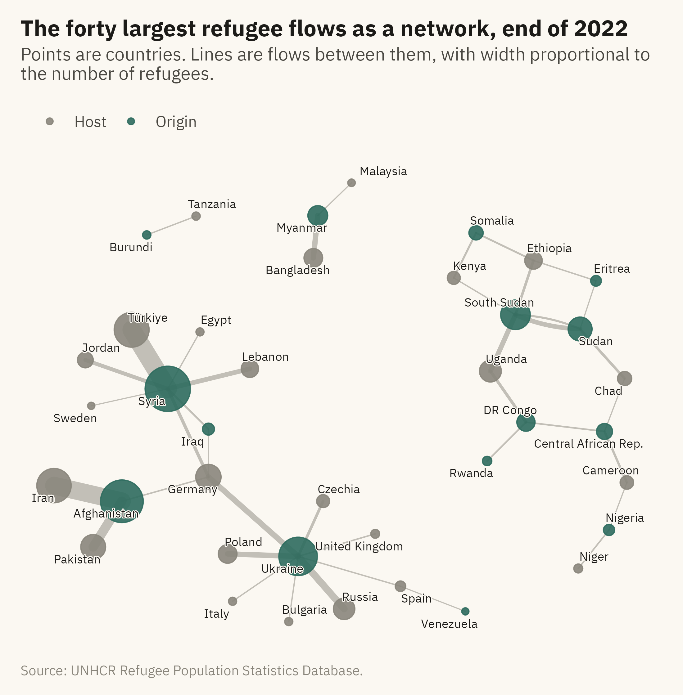
A network diagram answers a different question. It treats each country as a point, called a node, and each flow as a line between two points, called an edge. The question is no longer how large each flow is but how the countries are connected. Figure 4.9 draws the forty largest flows of 2022 as a network. Each edge is drawn with a width proportional to the flow, and each node is sized by the total number of refugees it hosts or sends.

edges <- w |> filter(year == 2022) |>
  group_by(origin, asylum) |> summarise(n = sum(refugees), .groups = "drop") |>
  slice_max(n, n = 40) |> rename(from = origin, to = asylum, weight = n)
g <- as_tbl_graph(edges, directed = TRUE) |>
  mutate(total = centrality_degree(weights = weight, mode = "all"),
         role = if_else(name %in% edges$from, "Origin", "Host"))
set.seed(4)
ggraph(g, layout = "fr", weights = NA, niter = 2000) +
  geom_edge_fan(aes(width = weight), color = mv_ink$mute, alpha = 0.5, lineend = "round") +
  geom_node_point(aes(size = total, color = role), alpha = 0.9) +
  geom_node_text(aes(label = name), size = 2.5, family = mv_font(), color = mv_ink$ink, repel = TRUE,
                 max.overlaps = 30, bg.color = mv_ink$canvas, bg.r = 0.12) +
  scale_edge_width(range = c(0.3, 5), guide = "none") +
  scale_size_area(max_size = 12, guide = "none") +
  scale_color_manual(values = c(Origin = mv_accent(), Host = mv_ink$mute), name = NULL) +
  labs(title = "The forty largest refugee flows as a network, end of 2022",
       subtitle = "Points are countries. Lines are flows between them, with width proportional to the number of refugees.",
       caption = mv_source(src)) +
  theme_mv_blank() +
  theme(panel.grid = element_blank(), legend.position = "top")

Figure 4.9: The forty largest refugee flows at the end of 2022 drawn as a network. Each point is a country, sized by the total number of refugees it sent or hosted among these flows. Each line is a flow, with width proportional to its size. Origins are in color and hosts in grey. Countries that are both, such as Sudan and DR Congo, are colored as origins. Source: UNHCR.

The network shows what the Sankey diagram and the bar chart do not. Most flows are between neighbors, so the diagram separates into regional clusters. Some countries appear in two roles. Sudan hosts refugees from South Sudan and Eritrea and sends refugees to Chad and South Sudan. DR Congo hosts refugees from Central African Republic and Rwanda and sends refugees to Uganda. In a bar chart of hosts or a bar chart of origins, these countries appear in one list or the other. In the network they appear once, with lines to their hosts and to their origins.

Two cautions apply to network diagrams. The first is that the position of each point is set by an algorithm, not by the data. The layout used here places connected points near each other and unconnected points apart. Distances between points have no units and should not be read as quantities. The second is that a network with many nodes becomes a tangle, as a line chart with many series does. Forty flows is near the limit for a printed page.

ImportantEthics Moment: The Category Called “Other”

Every composition chart in this chapter has a group called “all others.” In Figure 4.3 it includes more than a hundred host countries. In Figure 4.6 it is the set of unlabeled rectangles. The group is needed, because a chart of every host country would not fit on a page. It is also the part of the chart with the least detail. A country that hosts 2,000 Syrian refugees does not appear on the chart, and those refugees count in the same way as the 3.5 million in Türkiye. The subtitle or caption can say how many people were grouped as “all others” and where a reader can find the full list. Without that line, the reader has no way to know what was left out.

TipTry It Online

Same Data, Six Charts at viz.marginoferrormedia.com/apps contains the UNHCR data for any year from 2010 to 2022. Choose a question, comparison or composition. The app then draws the data as sorted bars, grouped bars, a dumbbell, a 100 percent stack, a dot plot, and a treemap. Each chart is paired with one finding that can be read from that form. Try to find a question that the treemap answers and the bar chart cannot.

WarningAI Reality Check: The Default Is a Pie

Ask a model for “a chart of refugees by host country,” and the first draft is often a pie with thirty slices and a legend longer than the chart. The word “by” is often treated as a composition request, and composition as a pie. A prompt that states the question tends to produce a better match. “Which ten countries host the most refugees” tends to produce sorted bars. “What share of the world’s refugees are in low-income countries” tends to produce two slices or one stacked bar. “How did the top eight origins change from 2012 to 2022” tends to produce a dumbbell. This chapter lists those questions and the form that matches each one.

4.10 Putting It All Together

Comparison and composition are different questions, and each calls for different chart forms. For comparison, sorted horizontal bars with labeled values are the default. Dumbbells show change between two moments. Dot plots fit more than about a dozen categories. For composition, a 100 percent stacked bar is suitable when the parts are few and in a fixed order. A pie is suitable only for two or three slices. A treemap shows how a whole with many parts is divided. Small multiples of bars show two levels at once. A Sankey diagram shows flows between two sets of categories, and a network diagram shows which categories are connected. In each case, the title states what the chart shows and the subtitle or caption states what was left out.

4.11 Looking Ahead

Chapter 5 covers distribution. A bar chart shows one number per category. A distribution chart shows every number. The question changes from “which is larger” to “what is typical, how much do the values vary, and who is at the edges.” The case is school spending and outcomes across districts, where an average across districts leaves out most of the variation.

4.12 Further Reading and References

Cleveland, W. S. (1994). The Elements of Graphing Data, 2nd edition. Hobart Press. The source of the dot plot and the argument for it.

Few, S. (2012). Show Me the Numbers, 2nd edition. Analytics Press. Chapter 6 on bar charts and the rules used here.

Shneiderman, B. (1992). Tree visualization with tree-maps: 2-d space-filling approach. ACM Transactions on Graphics, 11(1), 92–99. The original treemap.

Skau, D., and Kosara, R. (2016). Arcs, angles, or areas: Individual data encodings in pie and donut charts. Computer Graphics Forum, 35(3), 121–130. Evidence that readers of a pie chart judge by arc or area rather than by angle.

UNHCR (2023). Global Trends: Forced Displacement in 2022. The annual report that summarizes the data used in this chapter, with further composition charts drawn from the same data.

4.13 Key Terms

Comparison and composition. The two questions this chapter answers. How values compare with each other, and how a whole divides into parts.

Dumbbell chart. Two points per category joined by a line, so the line’s length is the change.

100 percent stacked bar. A bar scaled to a whole, with segments as shares, in a fixed order.

Dot plot. Values as points on a common scale, one row per category. Fits many categories in little ink.

Treemap. Nested rectangles sized by value, for the structure of a whole with many parts.

Small multiples. One panel per group with shared axes, so the reader compares across panels.

Sankey diagram. A chart of flows between two or more sets of categories, in which the width of each band is proportional to the size of the flow.

Network diagram. A chart of connections, in which each category is a point and each connection is a line. The positions of the points are set by a layout algorithm, not by the data.

4.14 Exercises

Check Your Understanding

1. State the four rules for a bar chart and say which one Figure 4.1 breaks on purpose.
2. Why is Ukraine’s change easier to see in the dumbbell in Figure 4.2 than in the grouped bars?
3. Figure 4.3 and the stacked area in Chapter 3 both stack. Name three design differences that make the first readable and the second not.
4. When is a pie chart acceptable? State the conditions as a rule you could apply without judgment.
5. A colleague wants a treemap to show that Germany hosts more refugees than Pakistan. What would you tell them?

Apply It

6. Using ch04-refugees-world.csv, draw the ten largest host countries in 2022 as sorted horizontal bars with labeled values. Then draw the same as a vertical bar chart with the axis and no labels. Write one sentence on what the reader loses in the second version.
7. Build a dumbbell chart of the ten largest host countries in 2012 and 2022. Which country’s line is longest? Which reversed direction?
8. Redraw Figure 4.3 with eight segments instead of four. Describe what happens to the reader’s ability to compare the third-largest host across rows.
9. Draw the dot plot in Figure 4.5 without color. Then add color by income group instead of region. Which grouping is clearer, and why?

Think Deeper

10. The chapter says not to show both counts and shares on one chart. Find or imagine a case where a reader needs both, and design the pair of charts that would serve them.
11. Figure 4.7 uses a shared horizontal scale. Argue the case for free scales, then say which you would choose for a report to a regional office in Africa.
12. The Ethics Moment asks for a line about who was left out. Write that line for Figure 4.6, with the number of countries and people it would name.