Every chart so far in this book was fixed. The author chose what to show, and the reader looked at it. An interactive chart lets the reader make some of those choices. A reader can hover to see a value, click to filter, drag to zoom, or pick a year. The author of an interactive chart therefore makes two kinds of decision. The first is what the chart shows when it opens. The second is what the reader is allowed to change.
The case in this chapter concerns the Inland Northwest, seven counties around Spokane, Washington. The region has about 5,300 active nonprofits, and 1,200 of them are in human services. The question is whether those organizations are located where the need is. The data has one row per ZIP code. Each row gives the population, the poverty rate, and the number of human-services organizations. The question can be answered with a fixed chart or with a dashboard. This chapter explains when each is the better choice.
11.2 What Interactivity Is For
Shneiderman (1996) summarized the purpose of interaction as “overview first, zoom and filter, then details on demand.” The phrase names three steps a reader can take with a chart that allows them. In the first step, the reader sees the whole dataset. In the second, the reader narrows the view to the part of interest. In the third, the reader asks for the values behind one mark. A fixed chart supports only the first step, with a caption for the rest. An interactive chart can support all three.
Interaction has a cost. Each step the reader can take is work the author would otherwise have done, and many readers will not do it. A dashboard with twelve filters and no default view shows most visitors nothing. For that reason, this chapter treats interaction as a layer added to a chart that already reads well on its own. The author still chooses what the chart shows first.
11.3 The Overview
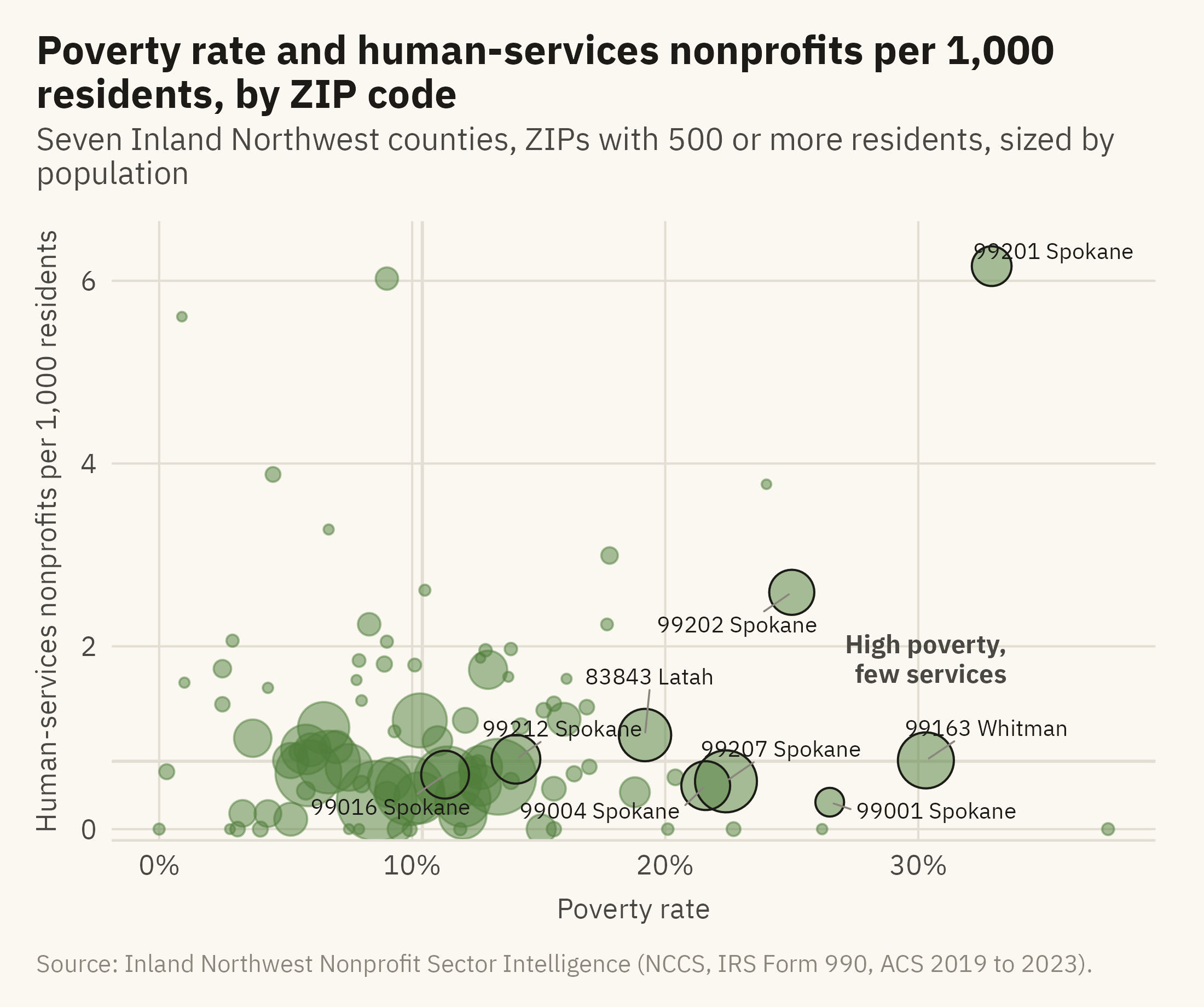
Figure 11.1 answers the question with a fixed chart. It has one point per ZIP code, with poverty rate on the horizontal axis and human-services organizations per thousand residents on the vertical axis. The points are sized by population.
Show the code
named <- g2 |>filter(zip %in%c("99201", "99207", "99163", "99001", "99004", "99202", "83843", "99016", "99212"))ggplot(g2, aes(poverty_rate, hs_per_1k)) +geom_hline(yintercept =median(g2$hs_per_1k), color = mv_ink$grid, linewidth =0.5) +geom_vline(xintercept =median(g2$poverty_rate), color = mv_ink$grid, linewidth =0.5) +geom_point(aes(size = population), color =mv_accent(), alpha =0.5) +geom_point(data = named, aes(size = population), color = mv_ink$ink, shape =21, stroke =0.5, fill =NA) +geom_text_repel(data = named, aes(label =paste0(zip, " ", county)), size =2.6, family =mv_font(), color = mv_ink$ink,min.segment.length =0, segment.color = mv_ink$mute, segment.size =0.3, box.padding =0.5, seed =4) +annotate("text", x =33.5, y =1.6, label ="High poverty,\nfew services", hjust =1, vjust =0, size =3, family =mv_font(), color = mv_ink$ink2, lineheight =0.95, fontface ="bold") +scale_size_area(max_size =12, guide ="none") +scale_x_continuous(labels =label_percent(scale =1)) +scale_y_continuous(expand =expansion(mult =c(0.02, 0.08))) +labs(title ="Poverty rate and human-services nonprofits per 1,000 residents, by ZIP code",subtitle ="Seven Inland Northwest counties, ZIPs with 500 or more residents, sized by population",x ="Poverty rate", y ="Human-services nonprofits per 1,000 residents",caption =mv_source(src)) +theme_mv(grid ="y") +theme(panel.grid.major.x =element_line(color = mv_ink$grid, linewidth =0.35))
Figure 11.1: ZIP codes in the seven-county Inland Northwest with at least 500 residents, by poverty rate and human-services nonprofits per 1,000 residents, sized by population. Downtown Spokane (99201) has the most organizations per resident and the highest poverty rate of any large ZIP. One small ZIP in Stevens County (99126) has a higher poverty rate and no organizations. The ZIPs in the lower right have high poverty and few organizations. Source: Inland Northwest Nonprofit Sector Intelligence (NCCS, IRS Form 990, ACS 2019 to 2023).
The two grey lines mark the medians and divide the chart into four quadrants. The lower right quadrant contains the ZIPs with high poverty and few organizations, which are the ZIPs the question asks about. Nine ZIPs are labeled because they are large, extreme, or both. This chart is the overview step in Shneiderman’s sequence. Every reader sees the same view, and the author has chosen it.
11.4 Details on Demand
Figure 11.2 is the same chart with the third step of Shneiderman’s sequence added. In the online edition, the reader can hover over any point. The hover shows the ZIP code, county, population, poverty rate, and count of organizations. In print, the figure shows the overview again without the labels, and the interaction is described only in this text.
Show the code
p <-ggplot(g2, aes(poverty_rate, hs_per_1k,text =paste0("ZIP ", zip, ", ", county, " County\nPopulation ", label_comma()(population),"\nPoverty rate ", poverty_rate, "%\n", n_human_services, " human-services organizations"))) +geom_hline(yintercept =median(g2$hs_per_1k), color = mv_ink$grid, linewidth =0.5) +geom_vline(xintercept =median(g2$poverty_rate), color = mv_ink$grid, linewidth =0.5) +geom_point(aes(size = population), color =mv_accent(), alpha =0.55) +scale_size_area(max_size =12, guide ="none") +scale_x_continuous(labels =label_percent(scale =1)) +labs(title ="Poverty rate and human-services nonprofits per 1,000 residents, by ZIP code", x ="Poverty rate", y ="Human-services nonprofits per 1,000 residents") +theme_mv(grid ="y") +theme(panel.grid.major.x =element_line(color = mv_ink$grid, linewidth =0.35))if (knitr::is_html_output(excludes ="epub")) { plotly::ggplotly(p, tooltip ="text") |> plotly::config(displayModeBar =FALSE) |> plotly::layout(font =list(family ="IBM Plex Sans, Inter, sans-serif"),paper_bgcolor = mv_ink$canvas, plot_bgcolor = mv_ink$canvas)} else { p +labs(subtitle ="Interactive in the online edition at viz.marginoferrormedia.com", caption =mv_source(src))}
Figure 11.2: The same chart with details on demand. Online, hovering over any point shows the ZIP code, county, population, poverty rate, and number of human-services organizations. The labels from the previous figure have been removed, because the reader can now ask for any of them. Source: Inland Northwest Nonprofit Sector Intelligence.
Hover is the cheapest interaction to add and is often the most useful. It addresses the labeling problem from Chapter 6. Any point can be labeled on request, and no label needs to be printed. One test applies to any hover. The chart should still be readable with the hover removed, as Figure 11.2 is in print. If the chart cannot be read without the hover, the author has not finished it.
11.5 Filter
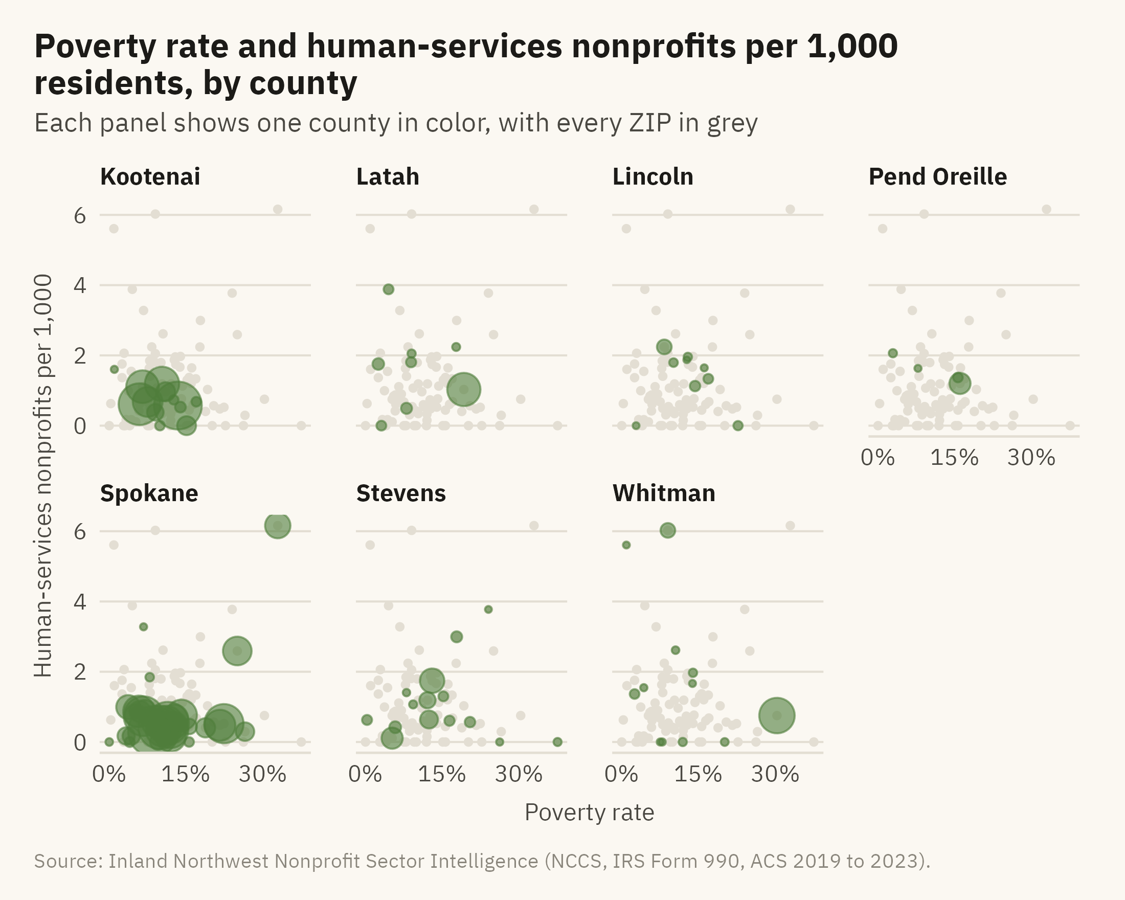
The second step, zoom and filter, lets the reader narrow the data to one part. In a fixed chart, the author does the filtering and shows the result as small multiples. Figure 11.3 shows the data filtered by county, with one panel per county.
Show the code
ggplot(g2, aes(poverty_rate, hs_per_1k)) +geom_point(data =select(g2, -county), color = mv_ink$grid, size =0.9) +geom_point(aes(size = population), color =mv_accent(), alpha =0.6) +facet_wrap(~ county, ncol =4) +scale_size_area(max_size =8, guide ="none") +scale_x_continuous(labels =label_percent(scale =1), breaks =c(0, 15, 30)) +labs(title ="Poverty rate and human-services nonprofits per 1,000 residents, by county",subtitle ="Each panel shows one county in color, with every ZIP in grey",x ="Poverty rate", y ="Human-services nonprofits per 1,000", caption =mv_source(src)) +theme_mv(base_size =10) +theme(strip.text =element_text(size =rel(0.85)))
Figure 11.3: The overview chart split by county, with all ZIPs in grey behind each panel. Spokane County has the most ZIPs, 33 of 94. The ZIPs with the highest coverage are small towns in Whitman, Latah, and Stevens, plus downtown Spokane. The one large point in Whitman County is Pullman, a university town with a high student poverty rate. Source: Inland Northwest Nonprofit Sector Intelligence.
A dropdown that selects one county at a time shows the reader one panel. Small multiples show all seven at once. When the filter has few values, the panels are usually the better choice, because the reader can compare the parts without clicking. A filter is more useful when the values are many, as with a hundred ZIP codes. It is also useful when the author cannot know in advance which part a reader wants.
11.6 Where: The Map Layer
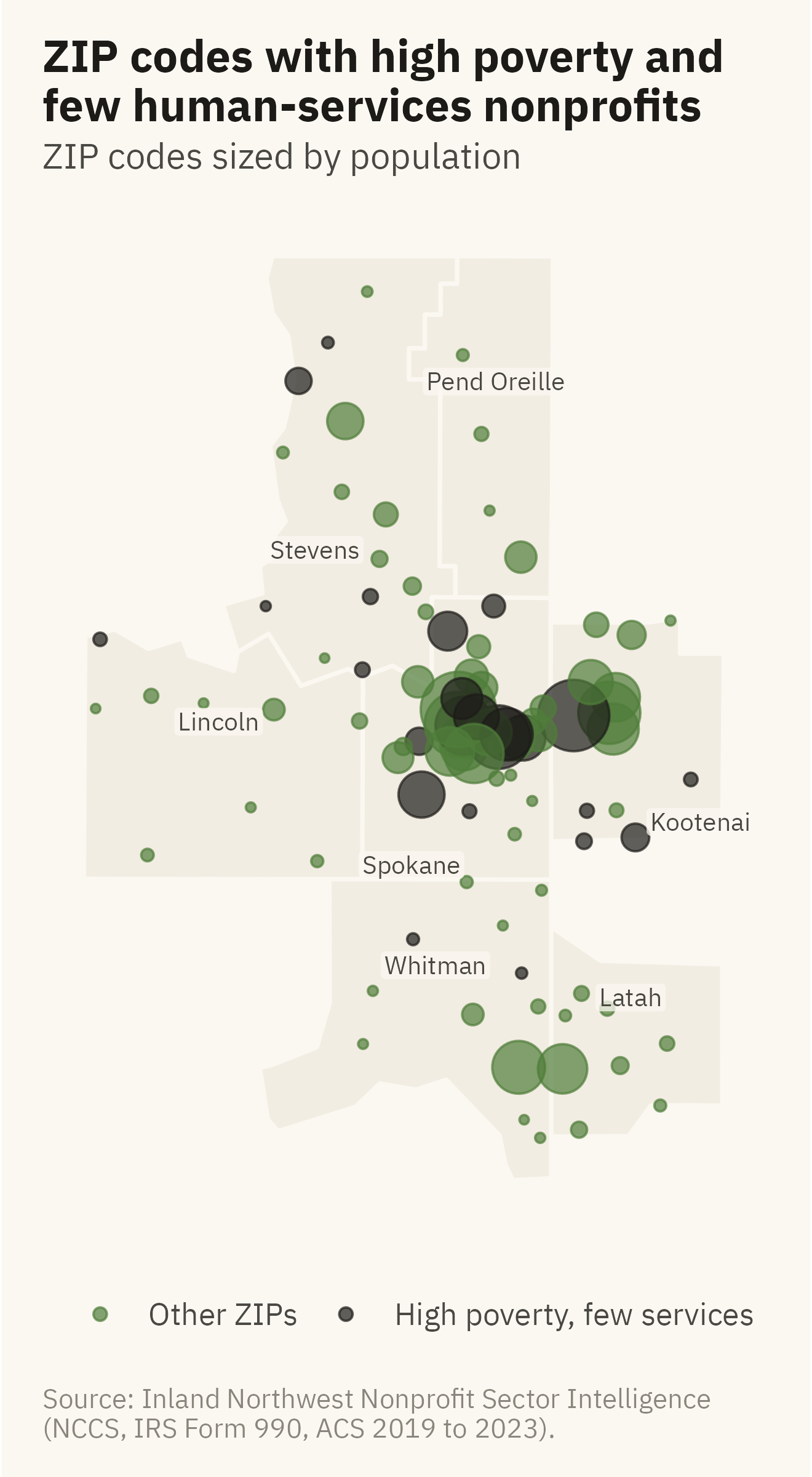
The question concerns location, so Figure 11.4 shows the ZIPs on a map of the region. In the online edition, the points have the same hover as Figure 11.2.
Show the code
cty_lab <-tribble(~county, ~lon, ~lat,"Kootenai", -116.42, 47.42, "Latah", -116.71, 46.93, "Lincoln", -118.42, 47.70,"Pend Oreille", -117.27, 48.65, "Spokane", -117.62, 47.30, "Stevens", -118.02, 48.18, "Whitman", -117.52, 47.02)ggplot() +geom_sf(data = inw, fill ="#F2EDE2", color = mv_ink$canvas, linewidth =0.6) +geom_point(data = g2, aes(lon, lat, size = population, color = gap), alpha =0.7) +geom_label(data = cty_lab, aes(lon, lat, label = county), size =2.6, family =mv_font(), color = mv_ink$ink2,fill =alpha(mv_ink$canvas, 0.75), label.size =0, label.padding =unit(0.12, "lines")) +scale_color_manual(values =c(`TRUE`= mv_ink$ink, `FALSE`=mv_accent()), labels =c("Other ZIPs", "High poverty, few services"), name =NULL) +scale_size_area(max_size =10, guide ="none") +coord_sf(default_crs =4326) +labs(title ="ZIP codes with high poverty and\nfew human-services nonprofits",subtitle ="ZIP codes sized by population",caption ="Source: Inland Northwest Nonprofit Sector Intelligence\n(NCCS, IRS Form 990, ACS 2019 to 2023).") +theme_mv_blank() +theme(legend.position ="bottom")
Figure 11.4: ZIP codes over the seven counties, sized by population and colored by whether they fall in the high-poverty, low-coverage quadrant of the overview chart. Twelve of the 25 dark points are in Spokane County, most of them in the Valley and on the north side. Five are in Kootenai County and eight are in the rural counties. Source: Inland Northwest Nonprofit Sector Intelligence; county boundaries from the US Census Bureau.
11.7 The Dashboard
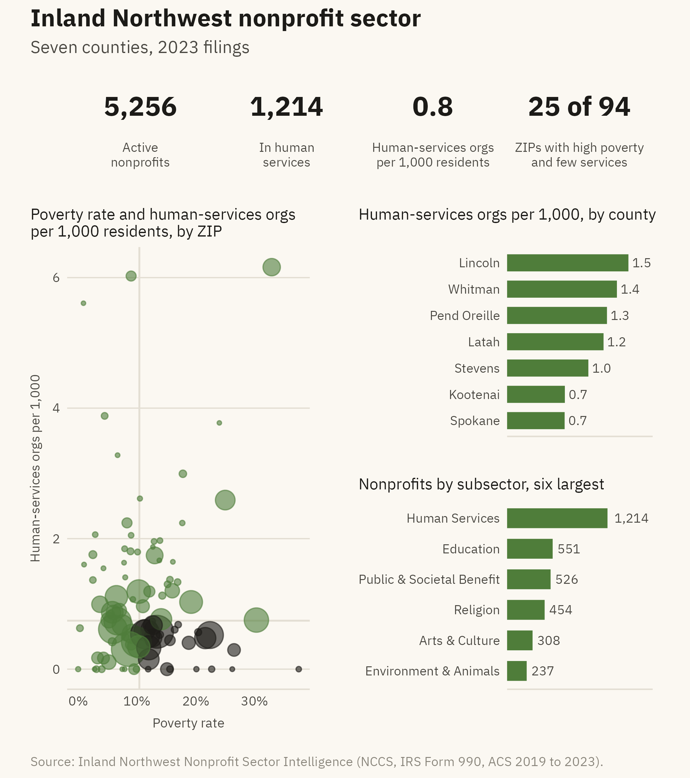
A dashboard is a page of charts meant to be read together. It is usually read more than once, often by someone who did not make it. The word comes from the instrument panel in front of a driver, where each gauge shows one quantity, such as speed or fuel. Each panel of a dashboard should likewise answer one question (Few, 2013). Figure 11.5 is a dashboard for the region’s nonprofit sector.
Show the code
tile <-function(value, label) {ggplot() +annotate("text", x =0, y =0.55, label = value, size =5.5, family =mv_font(), fontface ="bold", color = mv_ink$ink) +annotate("text", x =0, y =-0.5, label = label, size =2.6, family =mv_font(), color = mv_ink$ink2, lineheight =0.95) +scale_x_continuous(limits =c(-1, 1)) +scale_y_continuous(limits =c(-1.1, 1.3)) +coord_cartesian(clip ="off") +theme_void() +theme(plot.background =element_rect(fill = mv_ink$canvas, color =NA))}hs_zip <- gaps |>group_by(county) |>summarise(n_hs =sum(n_human_services), population =sum(population)) |>mutate(rate =1000* n_hs / population)hs <-sum(orgs$subsector =="Human Services"); tot <-nrow(orgs)k1 <-tile(label_comma()(tot), "Active\nnonprofits")k2 <-tile(label_comma()(hs), "In human\nservices")k3 <-tile(sprintf("%.1f", 1000*sum(hs_zip$n_hs) /sum(hs_zip$population)), "Human-services orgs\nper 1,000 residents")k4 <-tile(paste0(n_gap, " of ", nrow(g2)), "ZIPs with high poverty\nand few services")main <-ggplot(g2, aes(poverty_rate, hs_per_1k)) +geom_hline(yintercept =median(g2$hs_per_1k), color = mv_ink$grid, linewidth =0.5) +geom_vline(xintercept =median(g2$poverty_rate), color = mv_ink$grid, linewidth =0.5) +geom_point(aes(size = population, color = gap), alpha =0.6) +scale_color_manual(values =c(`TRUE`= mv_ink$ink, `FALSE`=mv_accent()), guide ="none") +scale_size_area(max_size =9, guide ="none") +scale_x_continuous(labels =label_percent(scale =1)) +labs(title ="Poverty rate and human-services orgs\nper 1,000 residents, by ZIP", x ="Poverty rate", y ="Human-services orgs per 1,000") +theme_mv(base_size =9) + plain_titlecty_bar <- hs_zip |>mutate(county =fct_reorder(str_remove(county, " County"), rate))side1 <-ggplot(cty_bar, aes(rate, county)) +geom_col(fill =mv_accent(), width =0.65) +geom_text(aes(label =sprintf("%.1f", rate)), hjust =-0.2, size =2.6, family =mv_font(), color = mv_ink$ink2) +scale_x_continuous(expand =expansion(mult =c(0, 0.2))) +labs(title ="Human-services orgs per 1,000, by county", x =NULL, y =NULL) +theme_mv(base_size =9, grid ="none") + plain_title +theme(axis.text.x =element_blank())sub <- orgs |>filter(subsector !="Unclassified") |>count(subsector, sort =TRUE) |>slice_head(n =6) |>mutate(subsector =fct_reorder(subsector, n))side2 <-ggplot(sub, aes(n, subsector)) +geom_col(fill =mv_accent(), width =0.65) +geom_text(aes(label =label_comma()(n)), hjust =-0.2, size =2.6, family =mv_font(), color = mv_ink$ink2) +scale_x_continuous(expand =expansion(mult =c(0, 0.45))) +labs(title ="Nonprofits by subsector, six largest", x =NULL, y =NULL) +theme_mv(base_size =9, grid ="none") + plain_title +theme(axis.text.x =element_blank())tiles <- (k1 | k2 | k3 | k4)body <- (main | (side1 / side2)) +plot_layout(widths =c(5, 3))(tiles / body) +plot_layout(heights =c(0.55, 2)) +plot_annotation(title ="Inland Northwest nonprofit sector", subtitle ="Seven counties, 2023 filings",caption =mv_source(src),theme = cap_theme +theme(plot.title =element_text(size =14, face ="bold", family =mv_font(), color = mv_ink$ink),plot.subtitle =element_text(size =10, family =mv_font(), color = mv_ink$ink2)))
Figure 11.5: A one-page dashboard for the Inland Northwest nonprofit sector. Four numbers run across the top, the main chart is at the left, and two supporting charts are at the right. Every panel answers one question and uses the chapter’s one accent color. The first two tiles and the subsector bars count all 5,256 registered organizations. The per-1,000 tile, the county bars, and the scatter use the 711 human-services organizations with a ZIP code in the data. Source: Inland Northwest Nonprofit Sector Intelligence.
The page follows five rules, most of them from Few (2013). They apply to any dashboard.
One question per panel. A panel designed to answer two questions is usually harder to read than two panels. Each of the four numbers across the top answers one question, and so does each chart.
The most important thing is largest and first. In languages read from left to right, readers tend to start at the top left of a page. The gap chart is the largest panel and the first chart below the tiles, because the page is about the gaps. The county bars and the subsector bars give context for it.
One color. When every panel has its own palette, a reader sees six separate charts on one page. With one accent color and grey in every panel, the reader sees one page.
Consistent units and scales. Both bar panels print their values and leave out the axis. The reader does not need to compare the two scales, which differ.
No gauges. Early business dashboards used speedometer dials and traffic lights. Each encodes a single number as an angle or a color, and Chapter 2 placed both encodings near the bottom of the Cleveland and McGill hierarchy. A gauge also takes space that a small chart could use to show a trend. A number in large type conveys the same value and is read more accurately.
11.8 Which Interactions to Add
The dashboard above is fixed. A reader of the online edition may want to know which ZIPs are the 25, which ZIPs are in the high-coverage cluster, or how the count has changed over time. Each question is a reason to add one interaction. The rule is to add the interaction the reader needs and no other.
Add a hover to identify a point, as in Figure 11.2. Add a single filter by county when readers are likely to care about their own county. Add a time slider when the data has years, which this data does not. A dashboard with a filter for every column is a query tool rather than a dashboard. A query tool is useful to the analyst who built it and to few other readers.
The online edition of this book has a companion app for every chapter’s data. The chapters are the fixed layer, and the apps are the interactive layer. Both are built from the same code, and the fixed layer is written first.
ImportantEthics Moment: A Number in a Tile
The dashboard reports in a tile, in large type, that 25 ZIP codes have high poverty and few services. The number depends on three choices. The thresholds are two medians chosen by the author. The count of registered organizations does not reflect their size or their hours. The poverty rate comes from a survey with its own margin of error. A different threshold gives a different count. The tile has no room for these qualifications, and dashboards rarely do. A number in a tile is likely to be repeated in a meeting as a settled fact. Before putting a number in a tile, ask whether it would still be fair if quoted without its caption. If not, show the chart instead of the tile.
TipTry It Online
Service Gaps at viz.marginoferrormedia.com/apps is the dashboard from this chapter with the three interactions described above. It has a hover on every point, a county filter, and a slider that moves the two thresholds. Move the thresholds and watch the count change. Then decide what number you would put in the tile.
WarningAI Reality Check: The Dashboard With Everything
Ask a model for a dashboard and the first draft often has a filter for every column, a chart for every variable, a color scheme for each chart, and at least one gauge. The model reproduces what the word “dashboard” means in its training data. Much of that output comes from business intelligence tools, and the defaults of those tools favor more panels and more controls.
Give the model the question first. A prompt such as “where are the gaps between need and services” tends to produce a page with one main chart and two supporting charts. Then ask for one interaction by name. A model can build a hover, a filter, or a slider when told which one to build. Without that instruction, it often builds all three and a dropdown.
11.9 Putting It All Together
Shneiderman’s sequence describes what a reader does with an interactive chart. The reader sees the whole, narrows to a part, and asks about one mark. Interaction should be added to a chart that already reads well without it. Hover is quick to add and is useful on most charts. A filter is an alternative to small multiples, and the panels are usually better when the filter has few values. A dashboard is a page of fixed charts, each answering one question. The most important chart comes first, the page uses one color, and single numbers appear in type rather than in gauges. The interactive layer is added last and kept small.
11.10 Looking Ahead
Chapter 12 takes one dataset from raw file to finished chart, using the methods from the whole book. The case is deaths that medical care could have prevented, by state. Most readers will not have seen a chart of that measure before. The chapter shows how to explain what the data shows without claiming more than the data supports.
11.11 Further Reading and References
Few, S. (2013). Information Dashboard Design: Displaying Data for At-a-Glance Monitoring, 2nd edition. Analytics Press. The source of most of the rules above, with a long catalogue of dashboards that break them.
Heer, J., and Shneiderman, B. (2012). Interactive dynamics for visual analysis. Communications of the ACM, 55(4), 45–54. A taxonomy of interactions and what each is for.
Patil, V. (2026). Inland Northwest Nonprofit Sector Intelligence. patilv.com/spokane-nonprofits. The source site for this chapter’s data, with the interactive versions of the charts.
Shneiderman, B. (1996). The eyes have it: A task by data type taxonomy for information visualizations. Proceedings of the IEEE Symposium on Visual Languages, 336–343. The overview, zoom and filter, details on demand sequence.
Wexler, S., Shaffer, J., and Cotgreave, A. (2017). The Big Book of Dashboards. Wiley. Worked examples of dashboards built for one question each.
11.12 Key Terms
Overview, zoom and filter, details on demand. Shneiderman’s sequence for what a reader does with an interactive chart.
Details on demand. A hover or click that shows the values behind a mark. The cheapest interaction and often the most useful.
Filter. An interaction that narrows the data to one part. An alternative to small multiples.
Dashboard. A page of charts read together, each answering one question, arranged by importance.
Tile. A single number in large type. It replaces the gauge and has the same risk of being quoted without context.
11.13 Exercises
Check Your Understanding
State Shneiderman’s sequence and match each step to one figure in this chapter.
The chapter says a chart that cannot be read without the hover is not finished. Explain what the test catches.
When is a filter better than small multiples, and when are the panels better?
List the five dashboard rules and identify one panel in Figure 11.5 that each rule shaped.
Why are gauges discouraged? Which chapter’s argument applies?
Apply It
Using ch11-zip-gaps.csv, redraw Figure 11.1 with organizations of all kinds rather than human-services organizations. Does the set of gap ZIPs change?
Move the two thresholds in the overview from the medians to the 75th percentile of poverty and the 25th percentile of coverage. How many gap ZIPs remain? Which tile number would you report?
Build a version of the dashboard for a single county, chosen with a filter. What panels change, and which become useless?
Add a hover to Figure 11.4 in the online edition and decide what five fields it should show.
Think Deeper
The chapter says the fixed layer is written first and the interactive layer is kept small. Describe a dataset and audience where the reverse would be right.
A funder wants a dashboard that updates every month. What would have to be true of the data pipeline for the count in the tile to mean the same thing each month?
The Ethics Moment asks whether a number would still be fair if quoted without its caption. Apply the test to each of the four tiles and say which pass.