In the spring of 1855, Florence Nightingale ran the nursing staff at a military hospital in Scutari, near Constantinople. Wounded and sick soldiers from the Crimean War were sent there to recover. Many of them died there instead. The wards were overcrowded. The sewers were broken and the water was contaminated. A building meant for a few hundred men held thousands. Soldiers who had survived the battlefield died of typhus, cholera, and dysentery in their beds. Nightingale kept records of the deaths and their causes.
She brought those records home in 1856 and took up the cause of army sanitation. The numbers supported her case. The officers and members of Parliament who controlled the money were unlikely to study tables of monthly death rates. She needed a form in which they could see the conclusion at once.
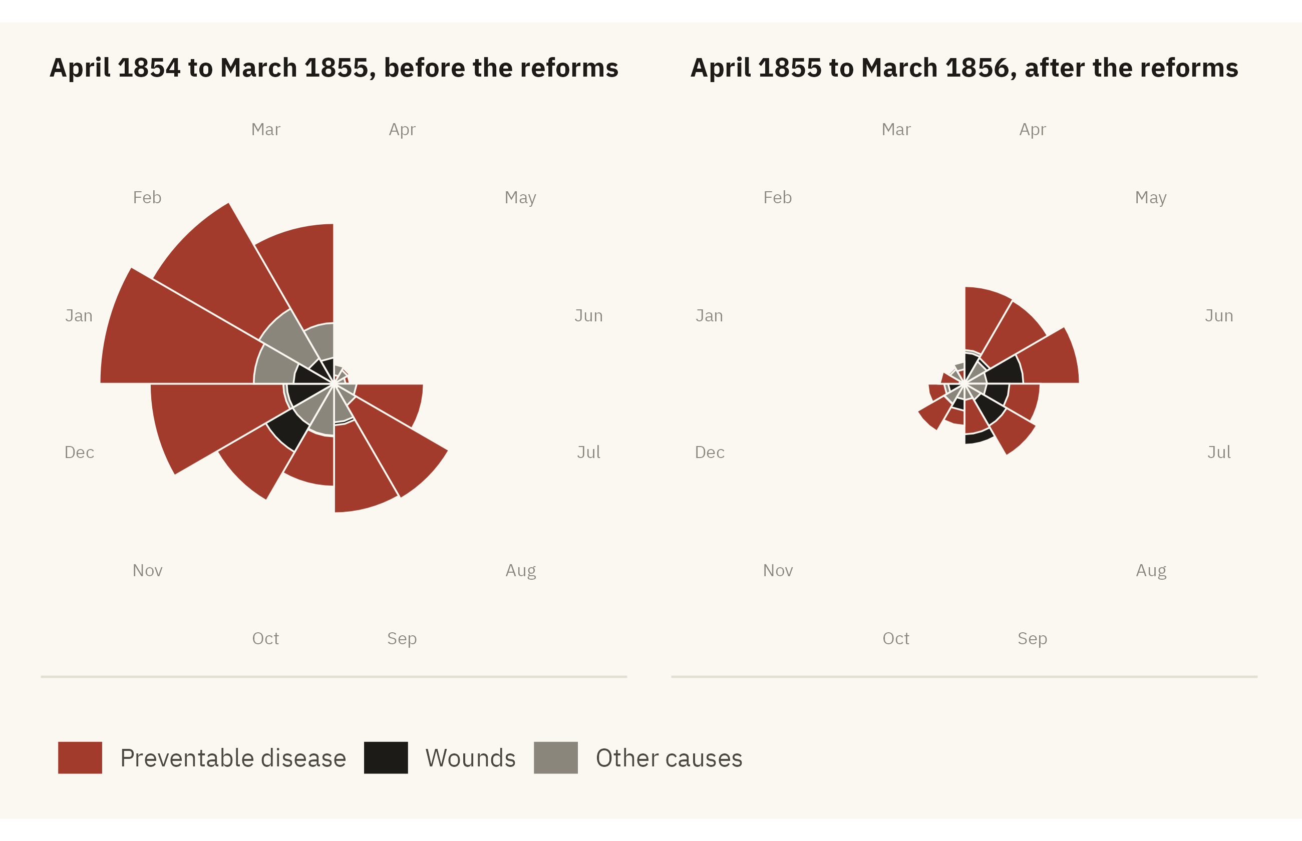
With help from the statistician William Farr, Nightingale drew a circular figure. She called it a “Diagram of the Causes of Mortality in the Army in the East.” Today it is usually called a polar-area chart, or a coxcomb. Each wedge is one month. The area of the wedge is the death rate in that month, split by cause. Deaths from preventable disease are one color. Deaths from wounds are another. Deaths from all other causes are a third.
Show the code
library(HistData)nightingale <- HistData::Nightingale |>mutate(Regime =if_else(Date <as.Date("1855-04-01"), "Before", "After"),Month =factor(format(Date, "%b"),levels =c("Apr","May","Jun","Jul","Aug","Sep","Oct","Nov","Dec","Jan","Feb","Mar"))) |>select(Month, Regime, Disease = Disease.rate, Wounds = Wounds.rate, Other = Other.rate) |>pivot_longer(c(Disease, Wounds, Other), names_to ="cause", values_to ="rate") |>mutate(cause =factor(cause, levels =c("Disease", "Wounds", "Other")),Regime =factor(Regime, levels =c("Before", "After"),labels =c("April 1854 to March 1855, before the reforms","April 1855 to March 1856, after the reforms")) ) |>arrange(Regime, Month, desc(rate))# Nightingale drew each cause from the center, not stacked, with the area of# each wedge proportional to the rate. A square-root radius keeps area proportional to the rate.ggplot(nightingale, aes(x = Month, y = rate, fill = cause)) +geom_col(position ="identity", width =1, color = mv_ink$canvas, linewidth =0.3) +coord_polar(start =0) +scale_y_sqrt() +scale_fill_manual(values =c(Disease =mv_accent(), Wounds = mv_ink$ink, Other = mv_ink$mute),labels =c("Preventable disease", "Wounds", "Other causes")) +facet_wrap(~ Regime, ncol =2) +labs(fill =NULL, x =NULL, y =NULL) +theme_mv(grid ="none") +theme(axis.text.y =element_blank(), legend.position ="bottom",axis.text.x =element_text(size =rel(0.7), color = mv_ink$mute),strip.text =element_text(hjust =0.5))
Figure 1.1: Florence Nightingale’s diagram of mortality in the British army, April 1854 to March 1856, redrawn from her data. Each wedge is one month, and its area is the annualized death rate per 1,000 soldiers. In nearly every month, deaths from preventable disease (dark red) are several times deaths from wounds (black). The right-hand circle covers the year after sanitary reforms began in March 1855, and it is smaller. Source: Nightingale (1858), via the HistData package.
In almost every month of the war, the wedge for disease is much larger than the wedges for wounds and other causes together. Soldiers were dying mainly from the conditions in the army’s own hospitals. In the worst months, more than seven times as many men died of disease as died of their wounds. The chart also shows what happened after the Sanitary Commission arrived in March 1855 and repaired the sewers and the water supply. The circle for the second year is much smaller than the first.
Nightingale sent the diagram to Queen Victoria, to the Secretary of State for War, and to other people with a vote. The Royal Commission on the Health of the Army was convened. The reforms it recommended were adopted over the next decade. Nightingale had the same numbers in tables, and the tables were accurate. In the diagram, a reader can compare the causes of death without doing any arithmetic.
This book treats a visualization as an argument made with data. A well-made visualization supports its claim when a reader checks the claim against the data.
1.2 The Number You Cannot See
Nightingale’s chart is 170 years old. The same difference between a table and a chart can be shown with a current series. This section presents one number first in a table and then in a chart.
The number is the share of children who die before their fifth birthday. The United Nations Inter-agency Group for Child Mortality Estimation (UN IGME) publishes it every year for every country. Gapminder has reconstructed it back to 1800 from parish records, censuses, and early national statistics. Table 1.1 shows the world figure at a few points in time.
Show the code
world |>filter(year %in%c(1800, 1860, 1900, 1940, 1960, 1980, 2000, 2017)) |>mutate(`Of every 100 children`=round(share_dying_pct)) |>select(Year = year, `Share dying before age five (%)`= share_dying_pct, `Of every 100 children`) |> knitr::kable(align ="lrr")
Table 1.1: Share of children worldwide who died before age five, selected years. Source: Gapminder and World Bank, compiled by Our World in Data.
Year
Share dying before age five (%)
Of every 100 children
1800
43.30
43
1860
41.40
41
1900
36.20
36
1940
23.90
24
1960
18.50
18
1980
11.64
12
2000
7.71
8
2017
3.91
4
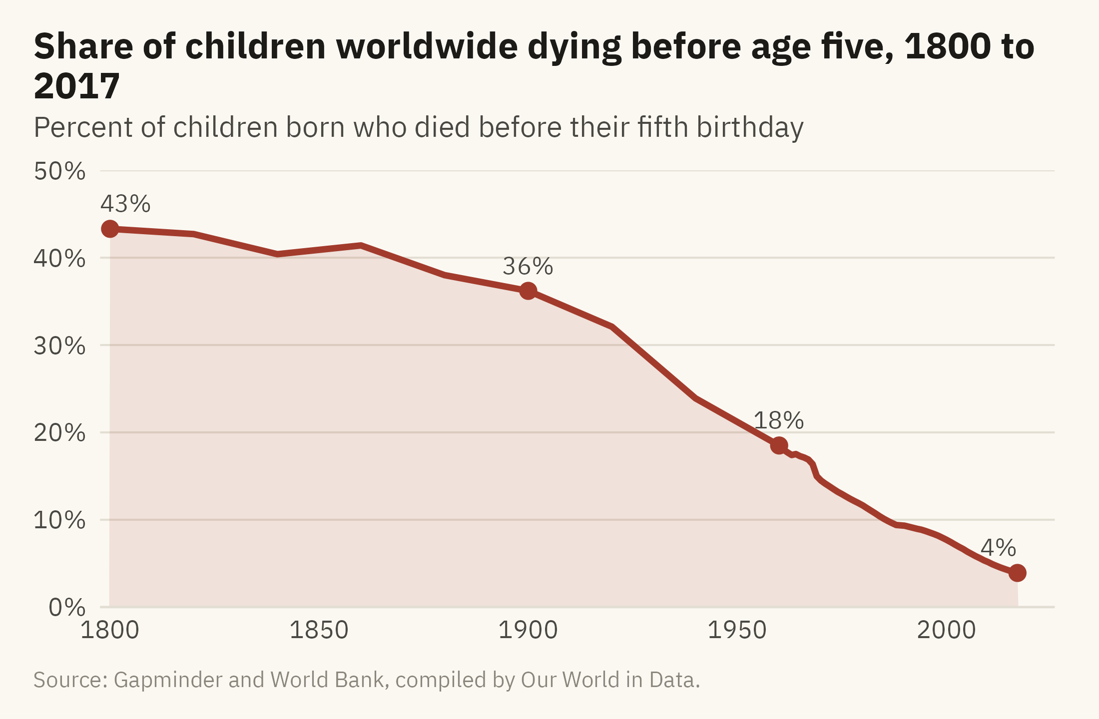
In 1800, 43 of every 100 children born did not reach the age of five. In 2017, 4 of every 100 did not. The share fell from 43 to 36 percent over the nineteenth century, and from 36 to 8 percent over the twentieth.
marks <- world |>filter(year %in%c(1800, 1900, 1960, 2017))ggplot(world, aes(year, share_dying_pct)) +geom_area(fill =mv_accent(), alpha =0.12) +geom_line(color =mv_accent(), linewidth =1.1) +geom_point(data = marks, color =mv_accent(), size =2.4) +geom_text(data = marks, family =mv_font(), size =3.1, color = mv_ink$ink2,aes(label =paste0(round(share_dying_pct), "%")),vjust =-1, hjust =c(0.2, 0.5, 0.5, 1)) +scale_x_continuous(breaks =seq(1800, 2000, 50), expand =expansion(mult =c(0.01, 0.04))) +scale_y_continuous(limits =c(0, 50), labels =label_percent(scale =1), expand =expansion(0)) +labs(title ="Share of children worldwide dying before age five, 1800 to 2017",subtitle ="Percent of children born who died before their fifth birthday",x =NULL, y =NULL,caption =mv_source("Gapminder and World Bank, compiled by Our World in Data")) +theme_mv()
Figure 1.2: Share of children worldwide who died before their fifth birthday, 1800 to 2017. The decline is slow through the nineteenth century, steep from about 1920, and steady after 1960. Source: Gapminder and World Bank, compiled by Our World in Data.
The table and the chart contain the same facts. A reader works with them differently. To read the table, you take in the values one at a time, 43 in 1800, 36 in 1900, 18 in 1960, and 4 in 2017, and work out the trend as you go. With the chart, you can see the trend before you read any single value. The decline was slow through the 1800s. The steepest fall came between 1920 and 1940. Since 1960 the line has fallen at a steady rate, about a quarter of a percentage point a year. The rate is now close to zero, so the line cannot fall much further.
A chart replaces a comparison that would need arithmetic with a visual judgment. Chapter 2 explains why visual judgment is faster than arithmetic and where it goes wrong. Some features of data, such as the shape of a decline over time, are present in a table but hard to read from it.
One Line Leaves Out 190 Countries
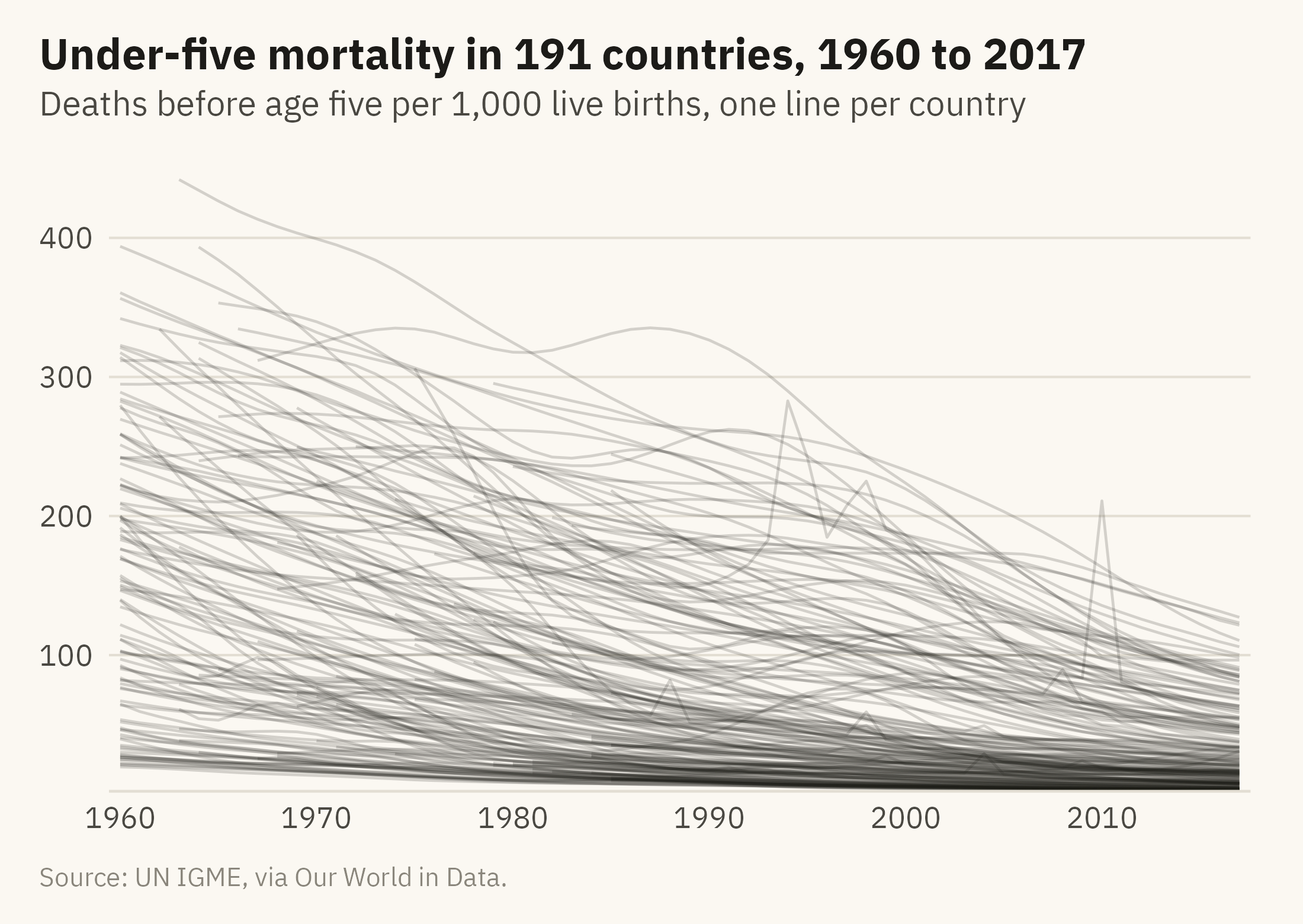
The world line is an average. A world average of 4 percent combines countries near 0.2 percent with countries near 13 percent. UN IGME publishes a figure for each country. Figure 1.3 plots all of them, one line per country, from 1960 to 2017.
Show the code
ggplot(u5, aes(year, under5_per_1000, group = country)) +geom_line(color = mv_ink$ink, alpha =0.18, linewidth =0.4) +scale_x_continuous(breaks =seq(1960, 2010, 10), expand =expansion(mult =0.01)) +scale_y_continuous(expand =expansion(mult =c(0, 0.04))) +labs(title ="Under-five mortality in 191 countries, 1960 to 2017",subtitle ="Deaths before age five per 1,000 live births, one line per country",x =NULL, y =NULL, caption =mv_source("UN IGME, via Our World in Data")) +theme_mv()
Figure 1.3: Under-five mortality rate for 191 countries, 1960 to 2017, one line per country. All but one line end lower than they start. Little else can be read from the figure, because no single line can be followed. Source: UN IGME, via Our World in Data.
Figure 1.3 shows that mortality fell in all but one country. The exception is Niue, a Pacific island with fewer than 2,000 people, where the rate rose from 11 to 22 per 1,000. The figure does not show where rates remain highest, how fast any one country improved, or whether the gap between the highest and lowest has narrowed, because no single line can be followed. Analysts call a line chart with this many series a spaghetti chart. It is a common first draft, in which all the data are drawn and no question has been chosen.
The next three figures draw the same data three ways. Each answers one question.
Where Are Children Still Dying?
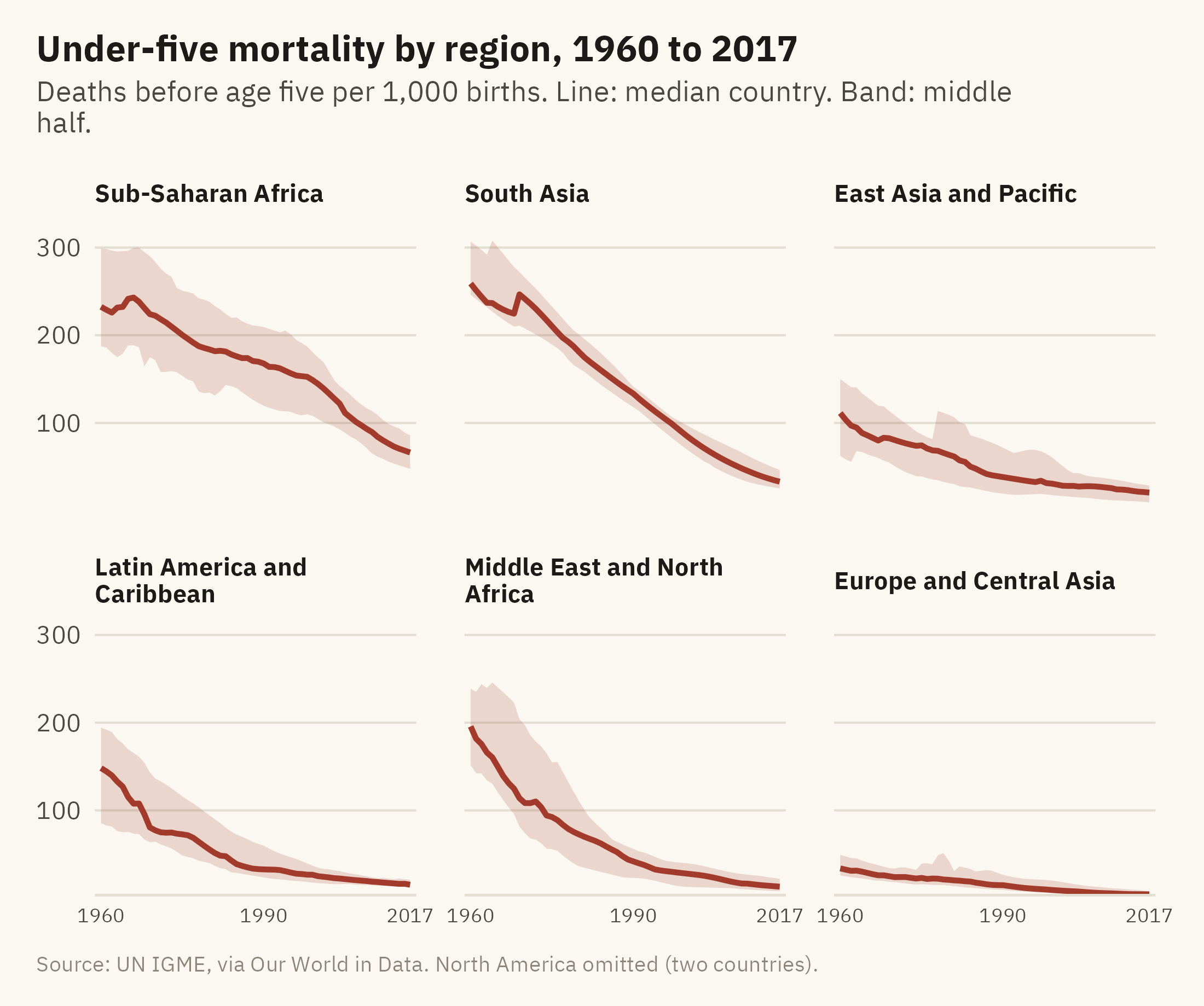
The first question is about place. Group the countries by World Bank region. Show each region’s spread as a band, with the median country drawn as a line.
Show the code
region_q <- u5 |>group_by(region, year) |>summarise(lo =quantile(under5_per_1000, 0.25),mid =median(under5_per_1000),hi =quantile(under5_per_1000, 0.75), n =n(), .groups ="drop") |>filter(n >=5) |>mutate(region =str_replace(region, " & ", " and "),region =fct_reorder(region, -mid, .fun = last))ggplot(region_q, aes(year)) +geom_ribbon(aes(ymin = lo, ymax = hi), fill =mv_accent(), alpha =0.18) +geom_line(aes(y = mid), color =mv_accent(), linewidth =0.9) +facet_wrap(~ region, ncol =3, labeller =label_wrap_gen(24)) +scale_x_continuous(breaks =c(1960, 1990, 2017), expand =expansion(mult =0.02)) +scale_y_continuous(expand =expansion(mult =c(0, 0.04))) +labs(title ="Under-five mortality by region, 1960 to 2017",subtitle ="Deaths before age five per 1,000 births. Line: median country. Band: middle half.",x =NULL, y =NULL, caption =mv_source("UN IGME, via Our World in Data","North America omitted (two countries)")) +theme_mv(base_size =10) +theme(axis.text.x =element_text(size =rel(0.8)), strip.text =element_text(size =rel(0.82)))
Figure 1.4: Under-five mortality by World Bank region, 1960 to 2017. The band covers the middle half of countries in each region (25th to 75th percentile) and the line is the regional median. Every region improved. South Asia started highest. Sub-Saharan Africa fell more slowly and has had the highest median since 1980. Its band is wide, so countries within the region differ as much as regions differ from each other. Source: UN IGME, via Our World in Data.
The six panels share one vertical axis, so a reader can compare heights across panels without reading the numbers. The panels are ordered by the 2017 median, highest first. South Asia, Sub-Saharan Africa, and the Middle East and North Africa start highest, with 1960 medians of 259, 232, and 196 deaths per thousand. All three fall. South Asia and the Middle East fall faster than Sub-Saharan Africa. By 2017, South Asia has reached about the level Europe had in 1960, and Sub-Saharan Africa has not. The width of the band for Sub-Saharan Africa is a second finding. Within that region, the countries at the 25th and 75th percentiles are further apart than the medians of Latin America and Europe. A chart of regional averages alone would not show that spread.
Who Improved Fastest?
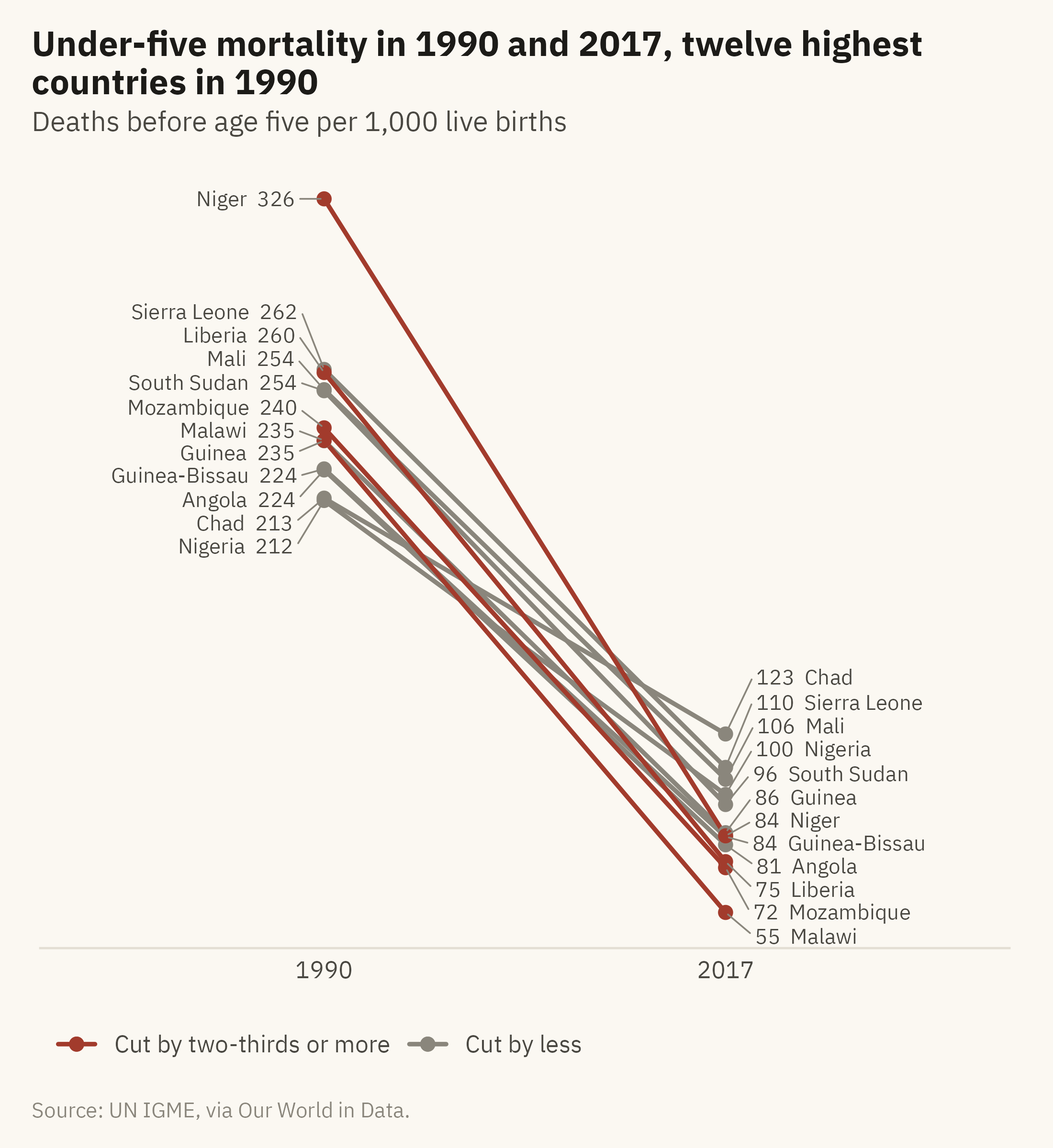
The second question is about change. Take the twelve countries with the highest mortality in 1990, the year the UN set its first child survival targets. Draw a line from each country’s 1990 value to its 2017 value.
Show the code
top12 <- u5 |>filter(year ==1990) |>slice_max(under5_per_1000, n =12) |>pull(country)slope <- u5 |>filter(country %in% top12, year %in%c(1990, 2017)) |>select(country, year, under5_per_1000) |>pivot_wider(names_from = year, values_from = under5_per_1000, names_prefix ="y") |>mutate(change = (y2017 - y1990) / y1990,fast = change <=-0.67) |>arrange(fast) # grey rows first, so the red lines and dots draw on topggplot(slope) +geom_segment(aes(x =1, xend =2, y = y1990, yend = y2017, color = fast),linewidth =0.8, lineend ="round") +geom_point(aes(x =1, y = y1990, color = fast), size =2) +geom_point(aes(x =2, y = y2017, color = fast), size =2) +geom_text_repel(aes(x =1, y = y1990, label =paste0(country, " ", round(y1990))),hjust =1, nudge_x =-0.08, direction ="y", size =2.8, family =mv_font(),color = mv_ink$ink2, segment.color = mv_ink$mute, segment.size =0.3,box.padding =0.1, min.segment.length =0) +geom_text_repel(aes(x =2, y = y2017, label =paste0(round(y2017), " ", country)),hjust =0, nudge_x =0.08, direction ="y", size =2.8, family =mv_font(),color = mv_ink$ink2, segment.color = mv_ink$mute, segment.size =0.3,box.padding =0.1, min.segment.length =0) +scale_x_continuous(limits =c(0.4, 2.6), breaks =c(1, 2), labels =c("1990", "2017")) +scale_y_continuous(expand =expansion(mult =0.05)) +scale_color_manual(values =c(`TRUE`=mv_accent(), `FALSE`= mv_ink$mute),breaks =c("TRUE", "FALSE"),labels =c("Cut by two-thirds or more", "Cut by less"), name =NULL) +labs(title ="Under-five mortality in 1990 and 2017, twelve highest countries in 1990",subtitle ="Deaths before age five per 1,000 live births",x =NULL, y =NULL, caption =mv_source("UN IGME, via Our World in Data")) +theme_mv(grid ="none") +theme(axis.text.y =element_blank(), legend.position ="bottom")
Figure 1.5: Under-five mortality in 1990 and 2017 for the twelve countries with the highest rates in 1990. Eleven of the twelve cut their rate by at least half, and Chad by 42 percent. Niger, Malawi, Liberia, and Mozambique cut theirs by more than two-thirds. Source: UN IGME, via Our World in Data.
A slope chart shows two points in time and the line between them. It leaves out the years in between, so the change is the only thing shown. The slope of each line is the rate of change. The lines are closer together at the right because the countries have converged. In 1990 they were spread between 210 and 330 deaths per thousand. In 2017 they were between 55 and 125. The four highlighted lines are the countries that improved fastest, and the highlight is the only color on the chart. Chapter 9 discusses this use of color. One color is applied to the four lines of interest, and the rest are grey.
How Far Apart Are Countries Today?
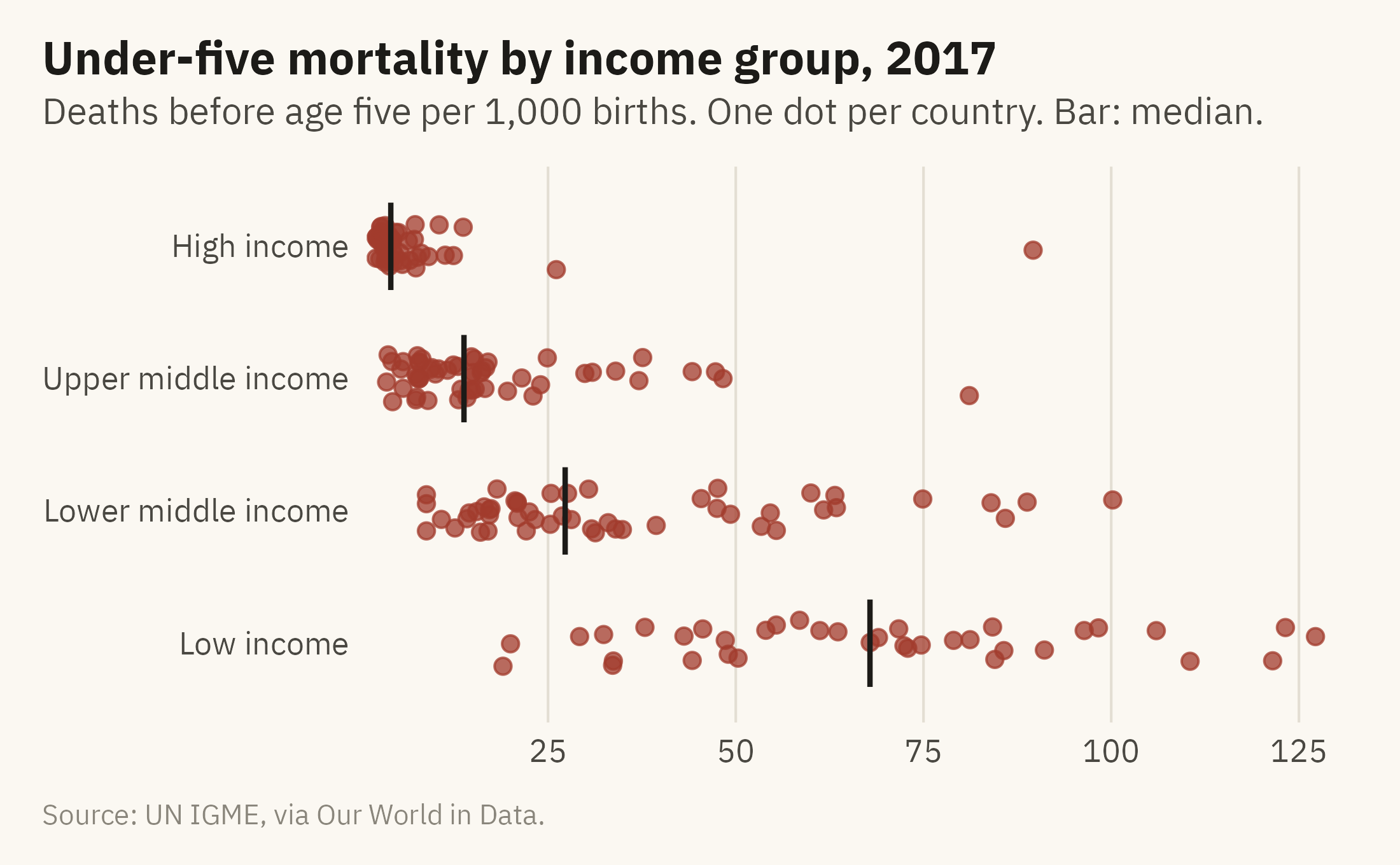
The third question is about the present, so the time axis can be dropped. Figure 1.6 places every country’s 2017 value on one axis, grouped by income.
Show the code
now <- u5 |>filter(year ==2017) |>mutate(income =factor(income, levels =c("High income", "Upper middle income","Lower middle income", "Low income")))set.seed(11)ggplot(now, aes(under5_per_1000, fct_rev(income))) +geom_jitter(height =0.18, width =0, size =1.9, alpha =0.75, color =mv_accent()) +stat_summary(fun = median, geom ="point", shape =124, size =7, color = mv_ink$ink) +scale_x_continuous(expand =expansion(mult =c(0.01, 0.03))) +labs(title ="Under-five mortality by income group, 2017",subtitle ="Deaths before age five per 1,000 births. One dot per country. Bar: median.",x =NULL, y =NULL, caption =mv_source("UN IGME, via Our World in Data")) +theme_mv(grid ="x")
Figure 1.6: Under-five mortality in 2017, one dot per country, grouped by World Bank income classification. The lowest-income group has the highest rates and the widest spread. The medians differ by income group, and the groups overlap. Source: UN IGME, via Our World in Data; income groups from Natural Earth.
The four charts come from one dataset. The world line shows the trend in the world average. The region panels show where rates are highest. The slope chart shows which countries improved most. The strip plot shows how far apart countries are in 2017. Each chart answers one question. The question was chosen first, and the chart was drawn to answer it. A reader can check the answer by looking at the chart.
ImportantEthics Moment: Whose Deaths Are Counted?
Every dot in Figure 1.6 is an estimate. Fewer than half the countries in the world register all births and deaths. For the rest, UN IGME fits a statistical model to household surveys, censuses, and whatever registration exists, and reports the model’s output as the country’s rate. In a country with a working registry, the deaths are counted. In a country without one, the deaths are estimated.
The chart is therefore a chart of estimates, and the estimates differ in precision. The countries with the least precise estimates tend to be the countries with the highest rates. In Figure 1.6, the dot for Sierra Leone and the dot for Sweden look alike, although one comes from a model and the other from a registry. Chapter 10 shows ways to display that difference. When a number describes people who were not individually counted, the chart should state where the number came from.
1.3 What a Visualization Is
The phrase data visualization is used for several different activities: making charts, exploring a dataset, building a dashboard, preparing a figure for a journal article, or producing the graphics in a newspaper. A definition that covers all of these is needed before the term can be used with care.
Robert Kosara (2016) offers a definition that is useful in practice. Kosara is a visualization researcher and was head of research at Tableau. For something to count as a visualization, three conditions must hold.
It is based on non-visual data. The starting point is information that is not a picture, such as death counts, sales figures, survey answers, sensor readings, or votes.
It produces an image. There is something to look at, on a screen, on paper, or on a wall.
The image is readable. A viewer can read the original data relationships back out of the picture. If the image distorts the data so that a reader cannot recover the original relationships, it fails this condition.
Misleading charts usually fail the third condition. Consider a bar chart with its baseline cut at 95, so that a change from 96 to 99 fills the frame. It has produced an image, and the image misrepresents the data. By Kosara’s definition it is a misuse of a visualization rather than a visualization. Most misleading charts meet the first two conditions and fail the third.
1.4 Three Jobs a Chart Can Do
Most charts serve one of three purposes: exploration, explanation, or persuasion. Each purpose calls for a different amount of care in the design.
The first job is exploration. An exploration chart is one you draw for yourself, to find out what the data look like, where the unexpected values are, and whether a relationship holds. The chart is quick to make and is usually discarded. Figure 1.3 was an exploration chart. It took a few lines of code and showed that nearly every country improved, and then it was set aside. An exploration chart does not need a finished title, chosen colors, or a source line. It does need to show the data accurately, because the analyst will make decisions based on it.
The second job is explanation. Once the analysis is done, you may need to report the finding to someone who did not do the analysis. An explanation chart takes more care. It needs a clean axis, a title that states the finding, a source line, and colors chosen for a reason. The region panels and the strip plot are explanation charts. Each presents one finding and has to be understood without the author present.
The third job is persuasion. When the goal is to change a decision, the chart is an argument, and readers who disagree with it will examine it. Nightingale’s coxcomb is a persuasion chart. She drew it for an audience that had reasons to resist its conclusion. The techniques that make a persuasion chart effective, such as a highlight or a title that states a claim, can also make it misleading. The slope chart in Figure 1.5 is close to persuasion. Four countries are highlighted in color, and the caption makes a claim about those four.
The same data can serve all three purposes. The amount of polish, the title, and the use of color should match the purpose of the chart.
1.5 Why You Cannot Skip the Picture
Readers who have taken statistics courses sometimes treat charts as decoration added after the analysis. The analyst computes the means and standard deviations, runs the test, and then makes a picture for the audience. Two well-known examples show why that order can lead to wrong conclusions.
Anscombe’s Quartet
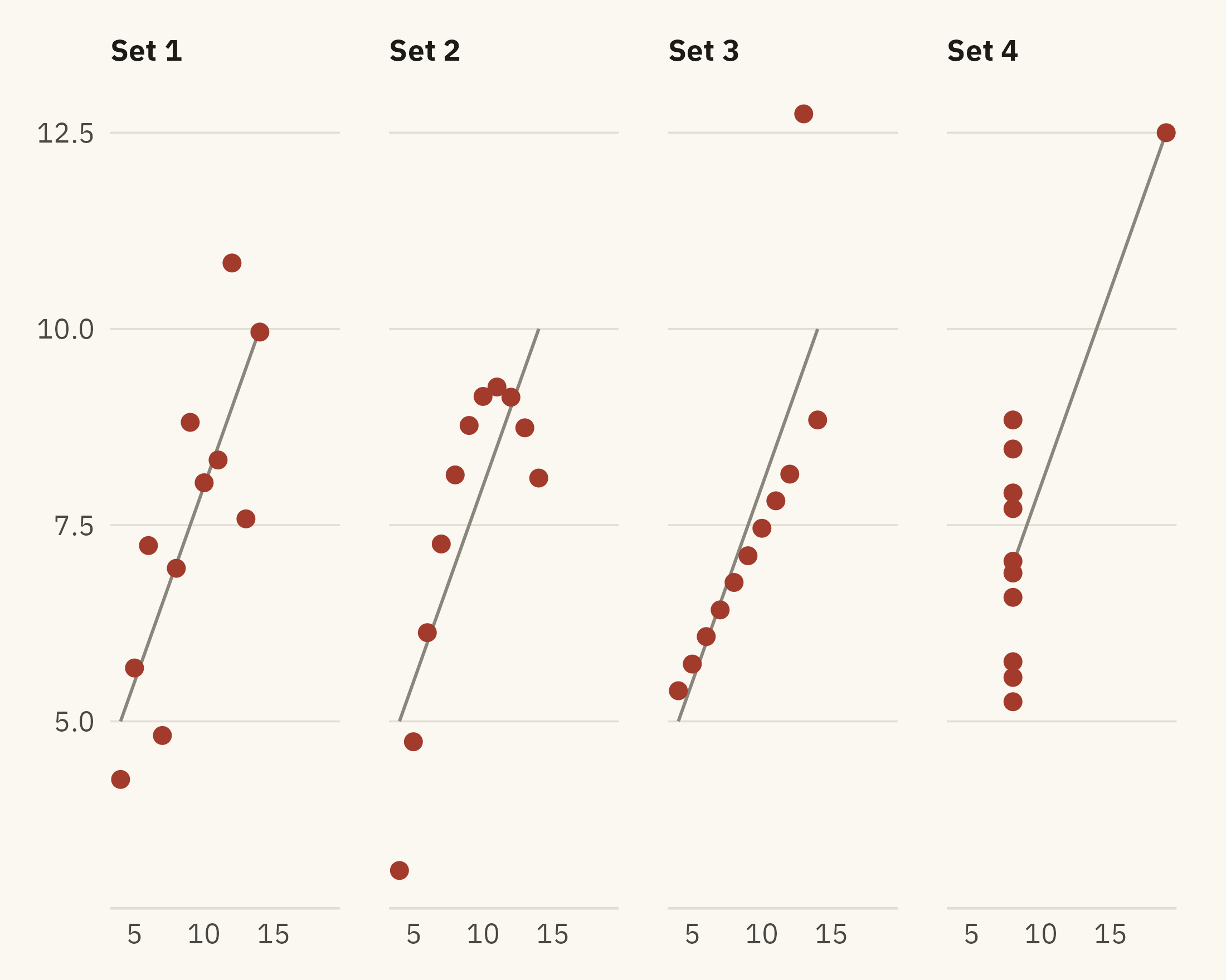
In 1973, the statistician Francis Anscombe published a short paper called “Graphs in Statistical Analysis.” He built four small datasets of eleven \((x, y)\) pairs each. To two decimal places, the four share the same mean of \(x\), the same mean of \(y\), the same variances, the same correlation, and the same regression line. The standard summaries do not distinguish them.
Table 1.2: Summary statistics for the four datasets in Anscombe’s Quartet. The four sets agree to two decimal places on every statistic shown.
Set
Mean x
Mean y
SD x
SD y
Correlation
1
9
7.5
3.32
2.03
0.82
2
9
7.5
3.32
2.03
0.82
3
9
7.5
3.32
2.03
0.82
4
9
7.5
3.32
2.03
0.82
Show the code
ggplot(anscombe_tidy, aes(x, y)) +geom_smooth(method ="lm", se =FALSE, color = mv_ink$mute, linewidth =0.5, formula = y ~ x) +geom_point(color =mv_accent(), size =2.2) +facet_wrap(~ set, ncol =4, labeller =as_labeller(\(s) paste("Set", s))) +scale_x_continuous(breaks =c(5, 10, 15, 20)) +labs(x =NULL, y =NULL) +theme_mv(grid ="none") +theme(panel.grid.major.y =element_line(color = mv_ink$grid, linewidth =0.3))
Figure 1.7: Anscombe’s Quartet. The four datasets share the summary statistics in the table above and the same fitted line, drawn in each panel. Set 1 is a linear relationship with scatter. Set 2 is a curve. Set 3 is a straight line with one outlier that changes the fitted slope. Set 4 has ten points at one value of x and one point elsewhere, and that one point produces the fitted line. Source: Anscombe (1973).
A statistician who reported the summaries without looking at the points would describe four different patterns with one sentence. Set 2 follows a curve, so a straight line is the wrong model for it. Set 3 is a straight line with one outlying measurement. Set 4 has no relationship among ten of its points, and the eleventh point produces the fitted line.
The Datasaurus Dozen
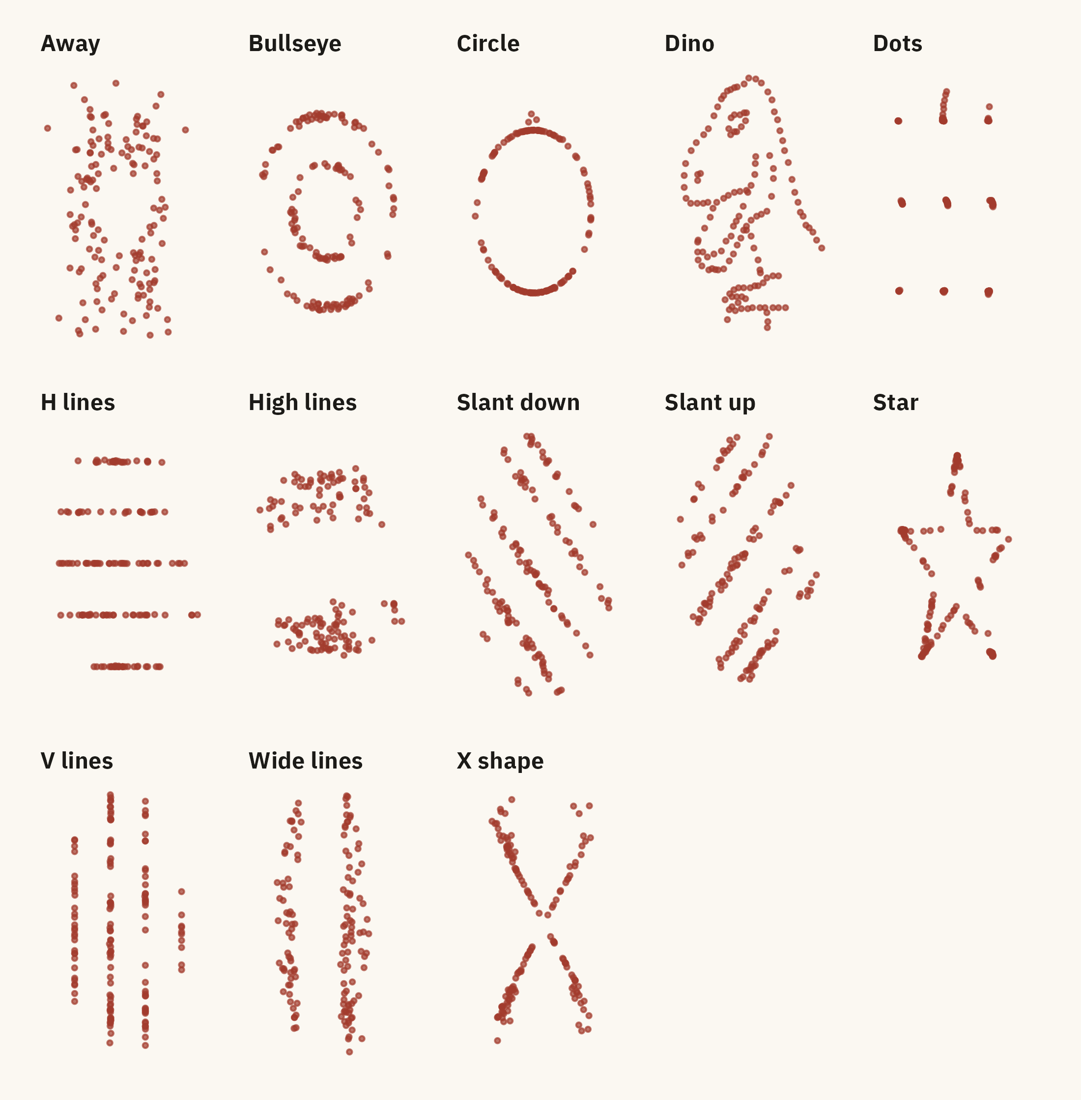
Justin Matejka and George Fitzmaurice (2017) extended Anscombe’s demonstration to thirteen datasets. Their paper, “Same Stats, Different Graphs,” used a search procedure to generate datasets that match on the mean of \(x\), the mean of \(y\), both standard deviations, and the correlation, all to two decimal places. The shapes include a star, a circle, a set of parallel lines, and a dinosaur.
Figure 1.8: The Datasaurus Dozen. Every panel has the same mean x, mean y, standard deviation of x, standard deviation of y, and correlation, to two decimal places. Source: Matejka and Fitzmaurice (2017), via the datasauRus package.
A summary table of these thirteen datasets would contain thirteen identical rows.
Summary statistics compress the data, and the compression removes information about shape. A chart shows that information. An analysis that uses summaries alone can miss a curve, an outlier, or a single point that produces a fitted relationship on its own.
Datasaurus Explorer lets you switch among the thirteen datasets while the summary statistics in the side panel stay frozen. Try to find two that look alike.
Child Mortality, Four Ways holds the UN IGME data from this chapter. Pick the countries, the years, and the question, and the app redraws the world line, the region panels, the slope chart, or the strip plot. Then try to make a chart that answers a question none of the four asked.
WarningAI Reality Check: Ask for the Picture
Give a language model a small dataset and ask what it shows. It often returns a sentence about the mean, the standard deviation, and the correlation. The numbers are usually right. Unless asked, the model does not usually draw the data and check the drawing against the summary. A model given Set 2 of Anscombe’s Quartet can report a correlation of 0.82 and describe the relationship as moderately strong and linear.
The same tools can draw a chart on request in seconds. The main risk is that the analyst accepts the summary before asking for the chart. A second risk is that the analyst examines a generated chart less carefully than one they drew themselves. Every chapter in this book includes a short section on what generated output means for the chapter’s subject. The rule from this chapter is to plot the data before relying on a summary of it.
1.6 Putting It All Together
This book treats a chart as an argument made with data. Nightingale’s diagram and the child mortality figures are a century and a half apart. In both, numbers that a reader would have to compute from in a table are drawn in a form the reader can compare by eye.
Three ideas from this chapter are used throughout the rest of the book. First, a visualization replaces arithmetic with visual judgment. Chapter 2 describes where that judgment is accurate and where it is not. Secondly, a chart answers one question, which the author chooses before drawing it. The spaghetti chart in Figure 1.3 shows only that nearly every country’s rate fell. Each of the four charts after it answers a more specific question. Third, plotting the data is part of the analysis, not a step after it. Anscombe’s Quartet and the Datasaurus Dozen show that datasets with the same summary statistics can have different shapes, and the shape determines whether the summary is a fair description.
1.7 Looking Ahead
Chapter 2 explains why the line in Figure 1.2 can be read faster than the table above it. The explanation comes from research on visual perception. It leads to rules about which visual encodings a reader can judge accurately and which they cannot. Those rules guide most of the chart choices in Part II.
1.8 Further Reading and References
Anscombe, F. J. (1973). Graphs in statistical analysis. The American Statistician, 27(1), 17–21. The original four datasets and the argument for plotting data before summarizing it.
Kosara, R. (2016). An empire built on sand: Reexamining what we think we know about visualization. Proceedings of the Sixth Workshop on Beyond Time and Errors on Novel Evaluation Methods for Visualization, 162–168. The source of the three-part definition used in this chapter.
Matejka, J., and Fitzmaurice, G. (2017). Same stats, different graphs: Generating datasets with varied appearance and identical statistics through simulated annealing. Proceedings of the 2017 CHI Conference on Human Factors in Computing Systems, 1290–1294. The Datasaurus Dozen paper.
Nightingale, F. (1858). Notes on Matters Affecting the Health, Efficiency, and Hospital Administration of the British Army. The diagram appears in the appendix. Friendly’s HistData package carries the data in machine-readable form.
Roser, M., Ritchie, H., and Dadonaite, B. (2019). Child and infant mortality. Our World in Data. The compiled historical series used in Figure 1.2, with notes on the Gapminder and World Bank sources.
UN Inter-agency Group for Child Mortality Estimation. Levels and Trends in Child Mortality. Annual report. The methods chapter explains how rates are estimated for countries without complete vital registration.
1.9 Key Terms
Polar-area chart. A circular chart in which each wedge spans an equal angle and its area encodes a value. Nightingale’s coxcomb is the best-known example.
Visualization. An image produced from non-visual data, from which a reader can recover the relationships in the data. Kosara’s definition.
Exploration, explanation, persuasion. The three jobs a chart does, in rising order of the care required.
Spaghetti chart. A line chart with so many series that no single one can be followed. It usually means that a question has not yet been chosen.
Small multiples. A grid of small charts with identical axes, one per group, so a reader can compare across panels. The region panels in this chapter.
Slope chart. A chart of two moments in time joined by a line per unit, so that change is the only thing shown.
Strip plot. One dot per observation along a single axis, often grouped. Shows a distribution without summarizing it.
Anscombe’s Quartet. Four datasets with identical summary statistics and different shapes. The standard demonstration that summary statistics do not determine the shape of the data.
1.10 Exercises
Check Your Understanding
Nightingale’s chart shows death rates per 1,000 soldiers, not counts of deaths. Why does that choice matter for comparing months in which the size of the army differed?
State Kosara’s three conditions for a visualization. Give an example of an image that meets the first two and fails the third.
Figure 1.3 and Figure 1.4 use the same data. Name two things a reader can learn from the second that are not available from the first.
Which of the three jobs (exploration, explanation, persuasion) does the slope chart do? What in its design tells you?
The four datasets in Anscombe’s Quartet have the same correlation. For which of the four is the correlation a fair summary of the relationship?
Apply It
Using the data file ch01-under5-by-country.csv from the companion site, make a slope chart for the twelve countries with the highest under-five mortality in 1960 rather than 1990. Which countries appear in both charts? Which improved faster in the earlier period?
Redraw the strip plot with regions in place of income groups. Write one sentence stating what the regional version shows that the income version does not, and one stating the reverse.
Compute the mean, standard deviation, and correlation for each of the thirteen datasets in the Datasaurus Dozen. Confirm that they match to two decimal places. Then choose any two datasets and describe, in words a reader without the chart could follow, how they differ.
The world line in Figure 1.2 has 65 points, one every twenty years up to 1960 and one a year after that. Plot the same series as a bar chart. Decide which form is better for this data and give one reason grounded in what the reader needs to judge.
Think Deeper
The Ethics Moment notes that most dots in Figure 1.6 are model estimates rather than counts. Propose two ways the chart could show a reader which countries have registration-based figures and which have estimates, and state one cost of each.
Nightingale chose a polar-area chart over a simple bar chart of the same monthly rates. Historians have argued the choice exaggerated the differences between months. Draw the bar chart version and decide for yourself. Was the coxcomb a fair persuasion chart or a misleading one?
A manager says, “Just give me the number. I don’t need a chart.” Using the child mortality data, write a short reply that names one specific decision the number alone would get wrong.