Since 1972, the General Social Survey has asked Americans one question in the same words every time. “Generally speaking, would you say that most people can be trusted, or that you can’t be too careful in dealing with people?” In 1972, 46 percent chose trust, and in 2018, 32 percent did. The World Values Survey asks the same question in about a hundred countries. The answers range from 74 percent in Norway to 3 percent in the Philippines.
The dataset is small and the finding is simple. This chapter uses it to cover the decisions that remain after the chart form has been chosen and the data checked. Those decisions concern color, type, and annotation. Software makes all three by default, and the default choices rarely fit the point a particular chart is meant to make.
9.2 Before and After
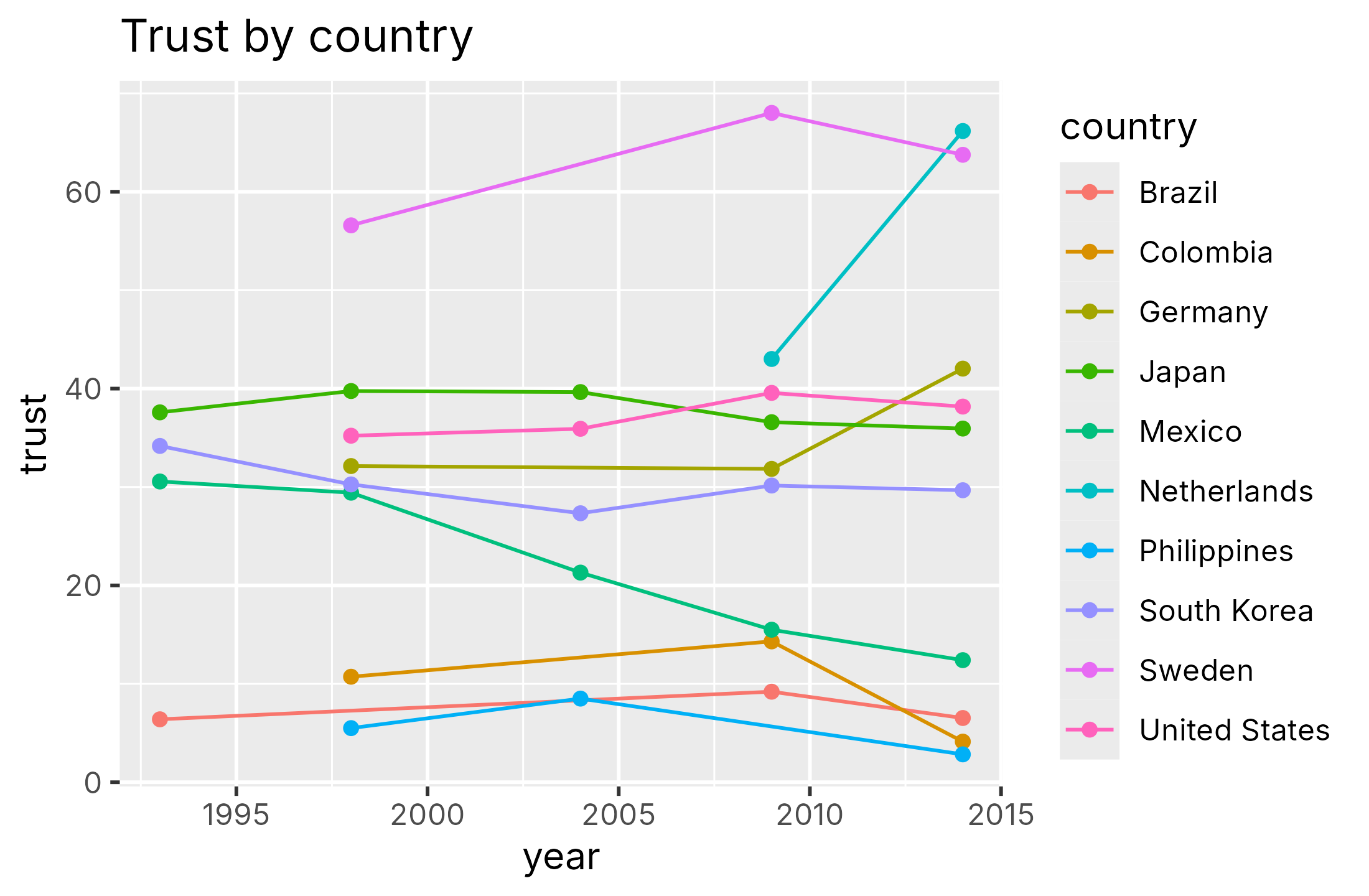
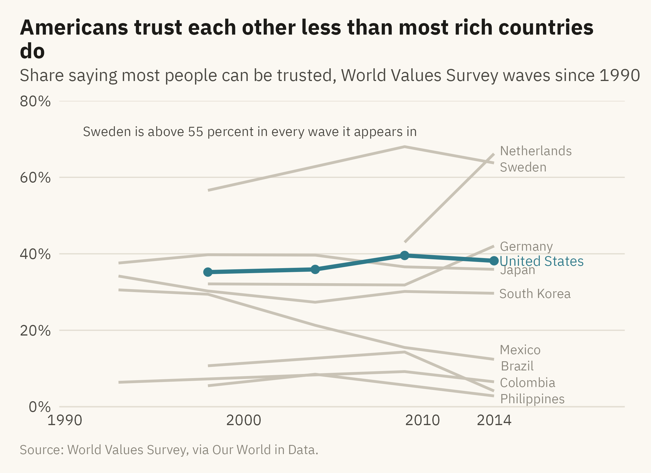
Figure 9.1 shows the trust data for ten countries as a plotting library draws it with no instructions. Figure 9.2 shows the same data after the color, type, and annotation have been chosen. The changes between the two charts are the subject of this chapter.
Show the code
old <-options(ggplot2.discrete.colour =NULL, ggplot2.discrete.fill =NULL)ggplot(wv10, aes(year, trust, color = country)) +geom_line() +geom_point() +labs(x ="year", y ="trust", color ="country", title ="Trust by country")
Figure 9.1: Share of people saying most people can be trusted, ten countries, World Values Survey waves since 1990, drawn with library defaults. The chart has ten hues, a legend, a grey panel, and a title that names the topic rather than a finding. Source: World Values Survey, via Our World in Data.
Show the code
ends <- wv10 |>group_by(country) |>slice_max(year, n =1) |>ungroup()ggplot(wv10, aes(year, trust, group = country)) +geom_line(data =filter(wv10, country !="United States"), color ="#C9C3B6", linewidth =0.8) +geom_line(data =filter(wv10, country =="United States"), color =mv_accent(), linewidth =1.2) +geom_point(data =filter(wv10, country =="United States"), color =mv_accent(), size =2) +mv_label_end(filter(ends, country !="United States"), aes(label = country), color = mv_ink$mute, nudge_x =0.4, size =2.8) +mv_label_end(filter(ends, country =="United States"), aes(label = country), color =mv_accent(), nudge_x =0.4, size =3) +annotate("text", x =1991, y =72, label ="Sweden is above 55 percent in every wave it appears in", hjust =0,size =2.9, family =mv_font(), color = mv_ink$ink2) +scale_x_continuous(breaks =c(1990, 2000, 2010, 2014), limits =c(1990, 2021), expand =expansion(mult =0.01)) +scale_y_continuous(labels =label_percent(scale =1), limits =c(0, 80), expand =expansion(0)) +labs(title ="Americans trust each other less than most rich countries do",subtitle ="Share saying most people can be trusted, World Values Survey waves since 1990",x =NULL, y =NULL, caption =mv_source(src_wv)) +theme_mv()
Figure 9.2: The same data after the color, type, and annotation have been chosen. One accent marks the United States, the other countries are grey, each line has a direct label, the title states the finding, and one annotation describes the series at the top. Source: World Values Survey, via Our World in Data.
The data are the same in both charts. Figure 9.2 has fewer colors, more words, and a title that states a finding. The next three sections cover those three changes in order.
9.3 Color
Chapter 2 gave the rules for color scales. Hue is suitable for categories, and intensity is suitable for ordered values. A diverging scale, with two hues that meet at a middle value, is suitable for values with a meaningful center. This section covers two further choices. The first is how many colors a chart should use. The second is whether every reader can tell the colors apart.
Fewer Hues Than Categories
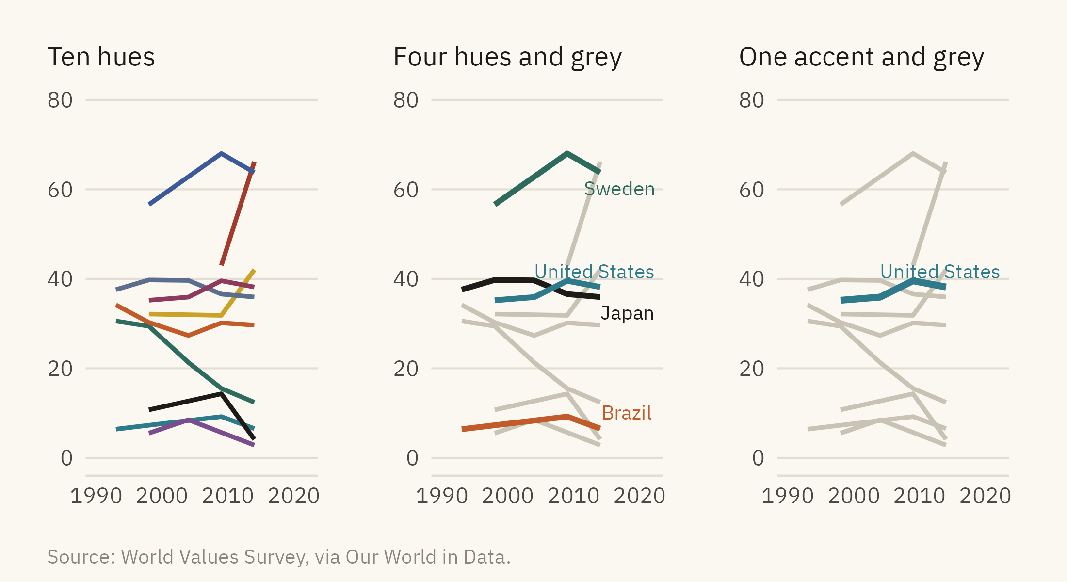
Readers can keep only a small number of hues apart without a legend, and a common working limit is six or seven. The number is smaller when the marks are thin lines. With ten countries in ten colors, the reader has to return to the legend for each line. A different palette does not change this. The better approach is to decide which categories the chart is about and to color only those. Figure 9.3 shows three options.
Show the code
h1 <-ggplot(wv10, aes(year, trust, color = country)) +geom_line(linewidth =0.8) +scale_color_manual(values =colorRampPalette(c(mv_accent(), "#1C1B18", "#C9A227", "#5B6E8C", "#2E6B5E", "#A23B2C", "#7A4E8C", "#C25B2A", "#3C5A99", "#8C3A5E"))(10), guide ="none") +scale_x_continuous(limits =c(1990, 2022)) +scale_y_continuous(limits =c(0, 80)) +labs(x =NULL, y =NULL, title ="Ten hues") +theme_mv(base_size =10) + plain_titlefour <-c("Sweden", "United States", "Japan", "Brazil")h2 <-ggplot(wv10, aes(year, trust, group = country)) +geom_line(data =filter(wv10, !country %in% four), color ="#C9C3B6", linewidth =0.8) +geom_line(data =filter(wv10, country %in% four), aes(color = country), linewidth =1) +mv_label_end(filter(ends, country %in% four), aes(label = country, color = country), nudge_x =0.3, size =2.6) +scale_color_manual(values =c(Sweden ="#2E6B5E", `United States`=mv_accent(), Japan ="#1C1B18", Brazil ="#C25B2A"), guide ="none") +scale_x_continuous(limits =c(1990, 2022)) +scale_y_continuous(limits =c(0, 80)) +labs(x =NULL, y =NULL, title ="Four hues and grey") +theme_mv(base_size =10) + plain_titleh3 <-ggplot(wv10, aes(year, trust, group = country)) +geom_line(data =filter(wv10, country !="United States"), color ="#C9C3B6", linewidth =0.8) +geom_line(data =filter(wv10, country =="United States"), color =mv_accent(), linewidth =1.2) +mv_label_end(filter(ends, country =="United States"), aes(label = country), color =mv_accent(), nudge_x =0.3, size =2.6) +scale_x_continuous(limits =c(1990, 2022)) +scale_y_continuous(limits =c(0, 80)) +labs(x =NULL, y =NULL, title ="One accent and grey") +theme_mv(base_size =10) + plain_titleh1 + h2 + h3 +plot_annotation(caption =mv_source(src_wv), theme = cap_theme)
Figure 9.3: Three ways to color ten series. Left, ten hues, which a reader cannot match to countries without a legend. Center, four hues for the countries the chart is about and grey for the rest. Right, one accent and grey, for a chart that makes one point. Source: World Values Survey, via Our World in Data.
Grey is the most useful color on a chart for a reason that follows from the figure and ground rule in Chapter 2. Grey lines are seen as background, so they keep the context visible without drawing attention. A single accent color against grey directs attention to one series. When every series has its own hue, no series stands out. This book uses one accent per chapter for that reason. Each accent was chosen to differ enough from grey and black that a reader can find it at once.
Color Every Reader Can Separate
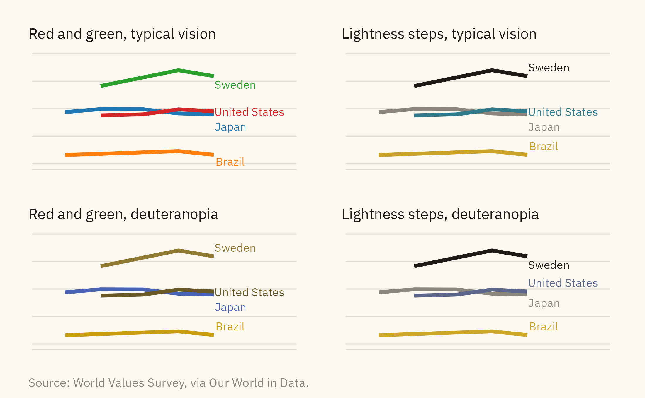
About one reader in twelve cannot tell red from green the way most readers can. Figure 9.4 shows two palettes two ways. The top row is how most readers see them. The bottom row is a simulation of deuteranopia, which is the most common form of color-vision deficiency.
Show the code
wv4 <-filter(wv10, country %in% four)e4 <-filter(ends, country %in% four)pal_bad <-c(Sweden ="#2CA02C", `United States`="#D62728", Japan ="#1F77B4", Brazil ="#FF7F0E")pal_good <-c(Sweden ="#1C1B18", `United States`=mv_accent(), Japan = mv_ink$mute, Brazil ="#C9A227")cvd <-function(pal, title) {ggplot(wv4, aes(year, trust, color = country)) +geom_line(linewidth =1.1) +mv_label_end(e4, aes(label = country, color = country), nudge_x =0.3, size =2.5) +scale_color_manual(values = pal, guide ="none") +scale_x_continuous(limits =c(1990, 2024)) +scale_y_continuous(limits =c(0, 80)) +labs(x =NULL, y =NULL, title = title) +theme_mv(base_size =9) + plain_title +theme(axis.text =element_blank())}(cvd(pal_bad, "Red and green, typical vision") +cvd(pal_good, "Lightness steps, typical vision")) / (cvd(deutan(pal_bad), "Red and green, deuteranopia") +cvd(deutan(pal_good), "Lightness steps, deuteranopia")) +plot_annotation(caption =mv_source(src_wv), theme = cap_theme)
Figure 9.4: Two palettes for four countries, as seen with typical color vision (top) and as simulated for deuteranopia, the most common red-green deficiency (bottom). In the simulation, the red and green on the left become two shades of the same olive. The colors on the right differ in lightness as well as hue, so a reader can still tell them apart. Source: World Values Survey, via Our World in Data; simulation after Machado, Oliveira, and Fernandes (2009).
Two tests can be run on any palette. The first is to convert it to grayscale. The second is to run it through a deficiency simulator. In both cases, check whether the categories can still be told apart. A palette whose colors differ in lightness as well as hue tends to pass both tests. A chart with direct labels passes both tests, because a label does not depend on color.
9.4 Type
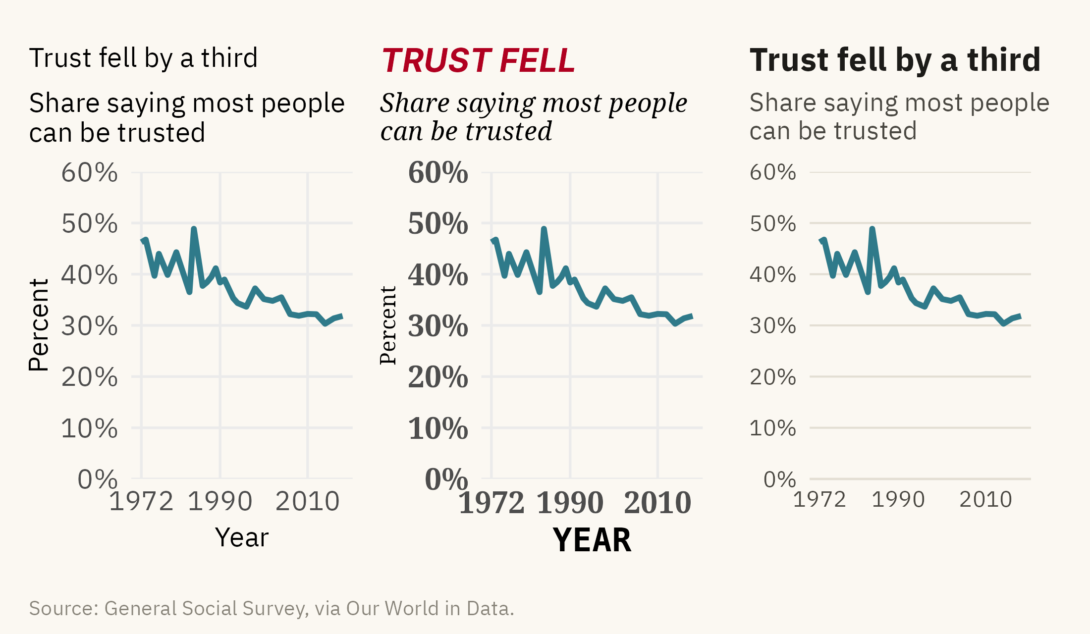
Every word on a chart has a size, a weight, and a color. These three settings decide which words a reader sees first. Most readers look at the largest and darkest text first. If that text is the axis title, the reader reads “year” before the title. Figure 9.5 shows the same chart with three treatments of type.
Show the code
base <-ggplot(us, aes(year, trust)) +geom_line(color =mv_accent(), linewidth =1) +scale_y_continuous(labels =label_percent(scale =1), limits =c(0, 60), expand =expansion(0)) +scale_x_continuous(breaks =c(1972, 1990, 2010))t1 <- base +labs(title ="Trust fell by a third", subtitle ="Share saying most people\ncan be trusted", x ="Year", y ="Percent") +theme_minimal(base_size =10, base_family =mv_font()) +theme(plot.title =element_text(size =10, face ="plain"), plot.subtitle =element_text(size =10), plot.title.position ="plot",axis.title =element_text(size =10), axis.text =element_text(size =10),plot.background =element_rect(fill = mv_ink$canvas, color =NA), panel.grid.minor =element_blank())t2 <- base +labs(title ="TRUST FELL", subtitle ="Share saying most people\ncan be trusted", x ="YEAR", y ="Percent") +theme_minimal(base_size =10, base_family ="serif") +theme(plot.title =element_text(size =12, face ="bold.italic", family ="sans", color ="#B00020"),plot.subtitle =element_text(size =9.5, face ="italic"), plot.title.position ="plot",axis.title.x =element_text(size =12, face ="bold", family ="mono"), axis.title.y =element_text(size =8),axis.text =element_text(size =11, face ="bold"), plot.background =element_rect(fill = mv_ink$canvas, color =NA),panel.grid.minor =element_blank())t3 <- base +labs(title ="Trust fell by a third", subtitle ="Share saying most people\ncan be trusted", x =NULL, y =NULL) +theme_mv(base_size =10)t1 + t2 + t3 +plot_annotation(caption =mv_source(src_us), theme = cap_theme)
Figure 9.5: The American trust series with three treatments of type. Left, every element is the same size and weight, so nothing is read first. Center, too many sizes, weights, and faces, so the red title and the bold axis title are read before the subtitle that says what is measured. Right, three levels. The bold title states the finding, the lighter subtitle says what is measured, and small grey text covers the axes and source. Source: General Social Survey, via Our World in Data.
Three levels are usually enough. The title is bold and the largest. The subtitle is one step smaller and lighter. Everything else is small and grey. Use one typeface, or two at most when the second is for numbers. Axis titles are often not needed. If the subtitle says “share saying most people can be trusted,” the vertical axis does not need the word “percent.” An axis labeled with years does not need the word “year.”
A title can name the topic or state the finding. “Trust by country” names the topic. “Americans trust each other less than most rich countries do” states a finding. Most figures in this book use a topic title and put the finding in the text, because a chapter supplies the sentence around each chart. A chart that will stand on its own, in a report or on a slide, usually does better with a finding title. A reader who sees only the title then knows what the chart found, and a reader who doubts the finding knows which numbers to check.
9.5 Annotation
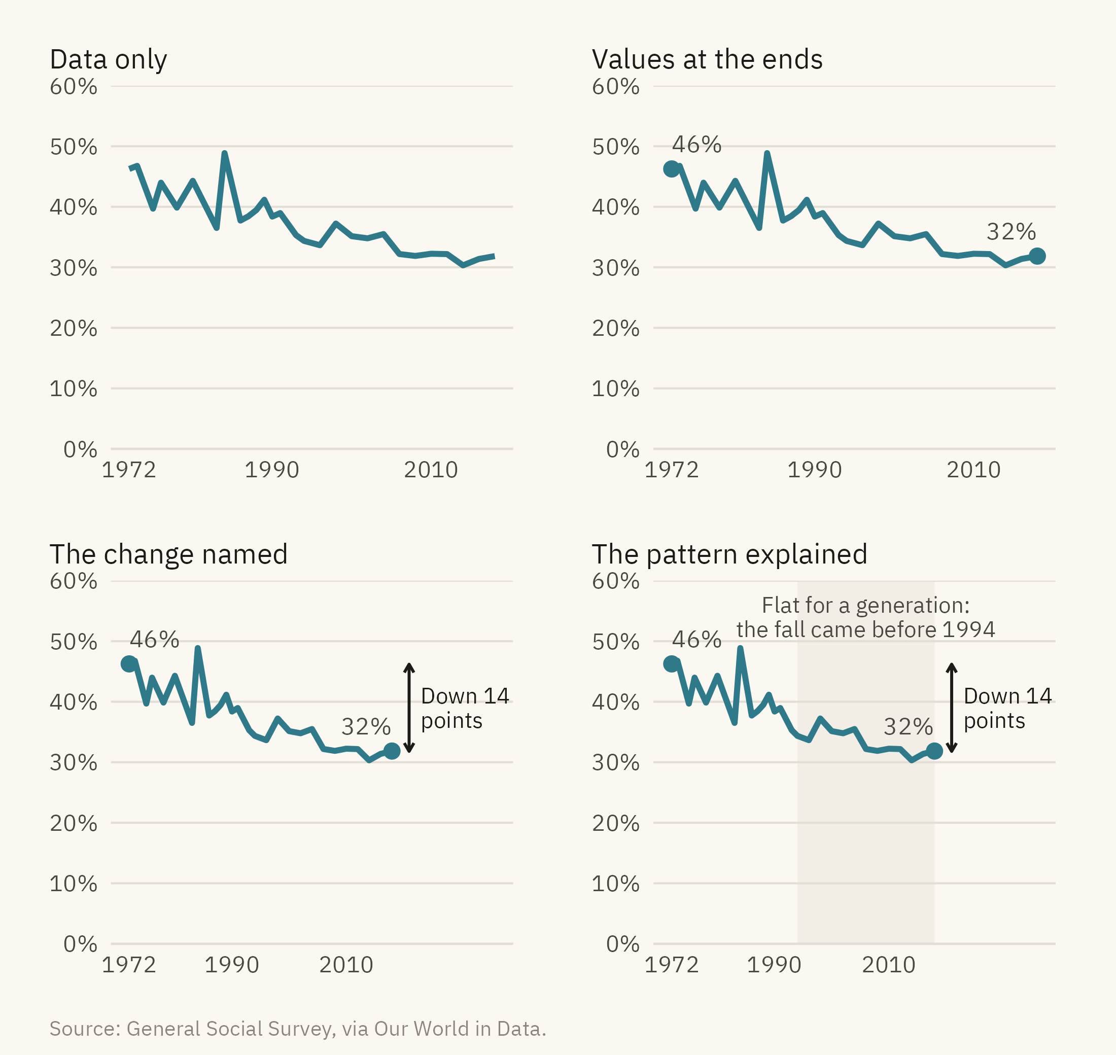
An annotation is a word or a mark placed on the chart to tell the reader what to look at. Adding one is quick and does not change the data. Figure 9.6 shows the American series four ways.
Show the code
pts <- us |>filter(year %in%c(1972, 2018))a0 <- base +labs(x =NULL, y =NULL, title ="Data only") +theme_mv(base_size =10) + plain_titlea1 <- base +geom_point(data = pts, color =mv_accent(), size =2.2) +geom_text(data = pts, aes(label =paste0(round(trust), "%"), hjust =c(0, 1)), vjust =-1, size =3, family =mv_font(), color = mv_ink$ink2) +labs(x =NULL, y =NULL, title ="Values at the ends") +theme_mv(base_size =10) + plain_titlea2 <- a1 +annotate("segment", x =2021, xend =2021, y =31.8, yend =46.2, color = mv_ink$ink, linewidth =0.5,arrow =arrow(ends ="both", length =unit(0.12, "cm"))) +annotate("text", x =2023, y =39, label ="Down 14\npoints", hjust =0, size =2.8, family =mv_font(), color = mv_ink$ink, lineheight =0.9) +scale_x_continuous(breaks =c(1972, 1990, 2010), limits =c(1972, 2036)) +labs(title ="The change named") + plain_titlea3 <- a2 +labs(title ="The pattern explained") + plain_titlea3$layers <-c(list(annotate("rect", xmin =1994, xmax =2018, ymin =0, ymax =60, fill = mv_ink$grid, alpha =0.4)), a3$layers)a3 <- a3 +annotate("text", x =2006, y =54, label ="Flat for a generation:\nthe fall came before 1994", size =2.8,family =mv_font(), color = mv_ink$ink2, lineheight =0.9)(a0 + a1) / (a2 + a3) +plot_annotation(caption =mv_source(src_us), theme = cap_theme)
Figure 9.6: The American trust series with no annotation, with the start and end values marked, with the change named, and with the change named and the long flat stretch explained. Each addition gives the reader more guidance about what to look at. None changes the data. Source: General Social Survey, via Our World in Data.
Annotations follow three rules. First, put the words near the thing they describe, and add a thin line to it if there is any doubt. Secondly, say what the reader should look at rather than what the chart contains. “Down 14 points” names a finding, and “Trust over time” only names the axes. Third, stop at three annotations. A pair of values that mark the two ends of a line counts as one. The last panel of Figure 9.6 has three: the end values, the arrow with its label, and the shaded band with its label. When a chart seems to need a fourth, the extra explanation usually belongs in the text around the chart.
9.6 Legends and Direct Labels
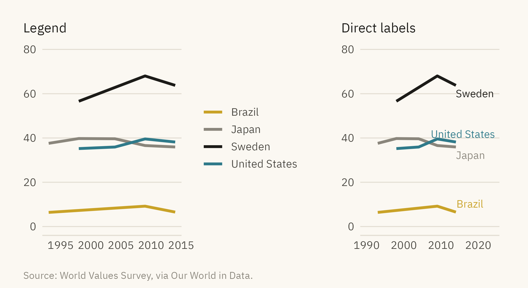
A legend is a table that matches each color to a name. The reader looks at a line, finds its color in the box, and reads the name. A direct label puts the name on the line itself. Each lookup in a legend interrupts reading and can produce a wrong match. Most charts in this chapter use direct labels for that reason. Figure 9.7 shows the difference.
Show the code
l1 <-ggplot(wv4, aes(year, trust, color = country)) +geom_line(linewidth =1) +scale_color_manual(values = pal_good, name =NULL) +scale_y_continuous(limits =c(0, 80)) +labs(x =NULL, y =NULL, title ="Legend") +theme_mv(base_size =10) + plain_title +theme(legend.position ="right")l2 <-ggplot(wv4, aes(year, trust, color = country)) +geom_line(linewidth =1) +mv_label_end(e4, aes(label = country, color = country), nudge_x =0.3, size =2.8) +scale_color_manual(values = pal_good, guide ="none") +scale_x_continuous(limits =c(1990, 2024)) +scale_y_continuous(limits =c(0, 80)) +labs(x =NULL, y =NULL, title ="Direct labels") +theme_mv(base_size =10) + plain_titlel1 + l2 +plot_annotation(caption =mv_source(src_wv), theme = cap_theme)
Figure 9.7: Four countries with a legend (left) and with direct labels at the end of each line (right). With the legend, the reader has to match four colors between the box and the lines. With direct labels, no matching is needed. Source: World Values Survey, via Our World in Data.
Legends are the better choice in two cases. One is when there are too many categories to label on the chart, as on a map. The other is when the color scale is continuous, as with a color ramp. Even then, the legend should be at the top, where most readers start. Its entries should be in the same order as the data.
9.7 The Finished Chart
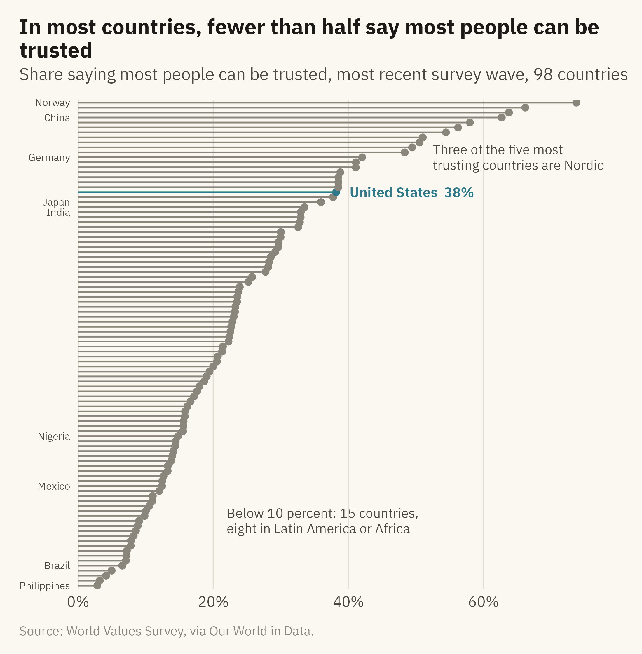
Figure 9.8 applies the rules in this chapter to the full world data. It contains 98 countries, one accent, three levels of type, two annotations, and a title that states a finding.
Show the code
latest <- wv |>group_by(country) |>slice_max(year, n =1) |>ungroup() |>mutate(country =fct_reorder(country, trust), us_flag = country =="United States")ggplot(latest, aes(trust, country)) +geom_segment(aes(x =0, xend = trust, yend = country, color = us_flag), linewidth =0.5) +geom_point(aes(color = us_flag), size =1.6) +geom_text(data =filter(latest, us_flag), aes(label =paste0("United States ", round(trust), "%")),hjust =0, nudge_x =2, size =3, family =mv_font(), color =mv_accent(), fontface ="bold") +annotate("text", x =52.5, y =87, label ="Three of the five most\ntrusting countries are Nordic", hjust =0,size =2.9, family =mv_font(), color = mv_ink$ink2, lineheight =0.95) +annotate("text", x =22, y =14, label ="Below 10 percent: 15 countries,\neight in Latin America or Africa", hjust =0,size =2.9, family =mv_font(), color = mv_ink$ink2, lineheight =0.95) +scale_color_manual(values =c(`TRUE`=mv_accent(), `FALSE`= mv_ink$mute), guide ="none") +scale_x_continuous(labels =label_percent(scale =1), expand =expansion(mult =c(0, 0.08))) +scale_y_discrete(labels = \(x) if_else(x %in%c("Norway", "China", "Germany", "Japan", "India","Mexico", "Nigeria", "Brazil", "Philippines"), x, "")) +labs(title ="In most countries, fewer than half say most people can be trusted",subtitle ="Share saying most people can be trusted, most recent survey wave, 98 countries",x =NULL, y =NULL, caption =mv_source(src_wv)) +theme_mv(grid ="x") +theme(axis.text.y =element_text(size =rel(0.7)), panel.grid.major.y =element_blank())
Figure 9.8: Share saying most people can be trusted in the most recent World Values Survey wave for each country, 98 countries sorted by value. The United States is marked. The Nordic countries, the Netherlands, and China are near the top. Most of Latin America and much of Africa are near the bottom. Source: World Values Survey, via Our World in Data.
ImportantEthics Moment: The Accent Points at One Country
A single accent color points at one thing. Figure 9.8 marks the United States because most readers of this edition are American. An edition for Brazil would mark Brazil, and the reader would take away a different finding. The title says that in most countries fewer than half trust other people, which is accurate. The annotation about Latin America and Africa is also accurate. Together, though, they can be read as a ranking of national character. The chart shows answers to one survey question. Those answers depend on history, inequality, and what the word “trust” means in about forty languages. The choices described in this chapter decide what the reader is directed to see. Before making them, decide whether the data support the sentence in the title, and consider what a reader in another country would take from the same chart.
TipTry It Online
Finish This Chart at viz.marginoferrormedia.com/apps starts with the default plot in Figure 9.1 and gives you the controls. You can set the number of highlighted series, the palette, a deficiency simulation, the type levels, the title, and up to three annotations that you drag into place. The app shows the grayscale version beside yours as you work.
WarningAI Reality Check: The Caption That Explains the Axes
A generated chart usually comes with a title that names the variables and a caption that explains the axes. Both are labels rather than findings. The model has not been told what the chart is for, so it cannot know what the reader should look at. Without that information, the title names the variables. “Trust by country, 1990 to 2014” is accurate and says nothing about what the chart found.
Tell the model the finding and ask for a title that states it. Ask for one accent and grey, and ask for direct labels. Ask it to remove any axis title that the subtitle already covers. Models tend to do all of this well when asked and little of it on their own.
9.8 Putting It All Together
The decisions in this chapter determine what a reader sees first and what the reader can ignore. One accent against grey directs attention to one series. A palette with lightness differences keeps the chart readable in grayscale and for readers with color-vision deficiency. Three levels of type place the finding in the title and the units in the subtitle, with no axis title that the subtitle already covers. Annotations name what the reader should look at, placed near the thing itself, with three as the usual limit. Direct labels replace a legend when the number of categories allows. None of these decisions changes the data.
9.9 Looking Ahead
Chapter 10 covers uncertainty. Every number in this book so far has been drawn as if it were exact. Survey shares, estimates, and forecasts all have ranges, and Chapter 10 shows how to draw them. The case is political polling, where the margin of error often matters as much as the reported number.
9.10 Further Reading and References
Brewer, C. A. (1994). Color use guidelines for mapping and visualization. In MacEachren, A. M., and Taylor, D. R. F. (eds.), Visualization in Modern Cartography, 123–147. Pergamon. The origin of the ColorBrewer palettes.
Cairo, A. (2016). The Truthful Art. New Riders. Chapters 8 and 9 on color and annotation.
Knaflic, C. N. (2015). Storytelling with Data. Wiley. A practical treatment of grey plus one accent, and of titles as findings.
Machado, G. M., Oliveira, M. M., and Fernandes, L. A. F. (2009). A physiologically-based model for simulation of color vision deficiency. IEEE Transactions on Visualization and Computer Graphics, 15(6), 1291–1298. The simulation used in Figure 9.4.
Stone, M. (2006). Choosing colors for data visualization. Perceptual Edge. A short guide to lightness as the first dimension to control.
9.11 Key Terms
Accent. The one color on a chart used to point at something. Everything else is grey or ink.
Direct label. The name of a series placed on or beside it, replacing a legend.
Type hierarchy. Three levels: title, subtitle, everything else. Size and weight decide what is read first.
Finding title. A title that states what the chart found, in a sentence with a verb.
Annotation. Words or marks on the chart that tell the reader what to look at. They go near the thing they describe, and three is the usual limit.
Color-vision deficiency. The inability to separate certain hues, most often red and green, affecting about one reader in twelve. Lightness differences and direct labels still work for these readers.
9.12 Exercises
Check Your Understanding
List every change between Figure 9.1 and Figure 9.2. Sort them into color, type, and annotation.
Why does the chapter call grey the most useful color on a chart?
State the three-level type hierarchy and say which element of Figure 9.5’s middle panel violates it most.
Rewrite these titles as findings: “Unemployment by state,” “Sales, 2020 to 2024,” “Survey results.”
When is a legend the right choice?
Apply It
Using ch09-trust-world.csv, draw the ten countries in Figure 9.1 with Brazil as the accent and write a title that states what the chart shows about Brazil.
Take any chart you have made and run it through a color-vision deficiency simulator. Record what separates and what collapses, and fix it with lightness or labels.
Add three annotations to Figure 9.8 that a reader would need, then remove the one that matters least and say why it was the one.
Set the same chart in three typefaces and judge which reads best at the size of a phone screen.
Think Deeper
The chapter argues for one accent. Describe a chart where two accents are needed, and the rule that would decide which two.
The Ethics Moment says the accent points at one country. Redesign Figure 9.8 so that no country is marked and the title still states a finding. What did the chart lose?
Annotation rule three says stop at three. Find a published chart with more than three and decide whether each one is needed.