In the 2016-17 school year, the United States had about 12,400 public school districts with at least 100 students. In the average district, 70 percent of students were white. That figure is correct, but it describes few actual districts. The average district has 3,700 students. The median district has 1,200. New York City has 920,000. A mean that counts each district once gives a rural district of 140 students the same weight as a city district of a million.
The figure changes when each district is weighted by its enrollment. Weighted that way, the share of students who attend a district that is mostly white is 49 percent, about twenty points below the district average. The average district is 70 percent white, and the average student’s district is 49 percent white. Both numbers come from the same table. They differ because the districts with the most students have the lowest shares of white students. An average that counts districts rather than students does not reflect that.
A single number is a summary of a distribution. This chapter covers charts that show the distribution instead of the summary. Three questions can be asked of any set of numbers. What is typical, how much the values vary, and which cases are at the edges. The case in this chapter is the racial makeup of American school districts.
5.2 One Variable: The Histogram
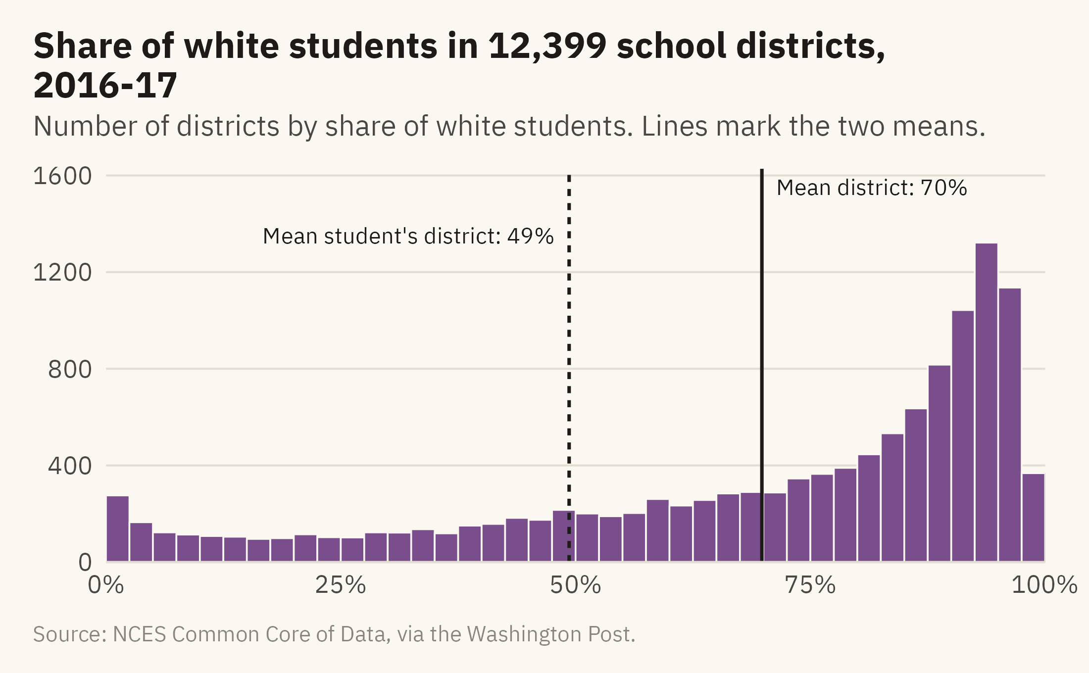
The histogram is the first chart to draw for any numeric variable. It sorts the values into bins and draws one bar per bin. The height of each bar is the count of values in that bin. Figure 5.1 shows the share of white students across all districts in 2016-17.
Show the code
ggplot(d17, aes(white)) +geom_histogram(binwidth =2.5, boundary =0, fill =mv_accent(), color = mv_ink$canvas, linewidth =0.3) +geom_vline(xintercept =mean(d17$white), color = mv_ink$ink, linewidth =0.6) +geom_vline(xintercept = w_mean, color = mv_ink$ink, linewidth =0.6, linetype ="22") +annotate("text", x =mean(d17$white) +1.5, y =1550, label ="Mean district: 70%", hjust =0,size =2.9, family =mv_font(), color = mv_ink$ink) +annotate("text", x = w_mean -1.5, y =1350, label =paste0("Mean student's district: ", round(w_mean), "%"),hjust =1, size =2.9, family =mv_font(), color = mv_ink$ink) +scale_x_continuous(labels =label_percent(scale =1), expand =expansion(0)) +scale_y_continuous(expand =expansion(mult =c(0, 0.05))) +labs(title ="Share of white students in 12,399 school districts, 2016-17",subtitle ="Number of districts by share of white students. Lines mark the two means.",x =NULL, y =NULL, caption =mv_source(src)) +theme_mv()
Figure 5.1: Share of white students in each of 12,399 school districts, 2016-17, in bins of 2.5 points. Most districts are near 90 percent, and a long tail runs toward zero. The district mean (70) and the student-weighted mean (49) are marked. Neither falls where most districts are. Source: NCES Common Core of Data, via the Washington Post.
The distribution is not symmetric around the mean. Most districts are near 90 percent, and the counts fall off slowly toward zero. Most districts have a higher share of white students than the national student body. A smaller number of large districts enroll most of the students of color. The mean of 70 falls in a low part of the distribution, and few districts have a value near it.
Bin Width Is a Choice
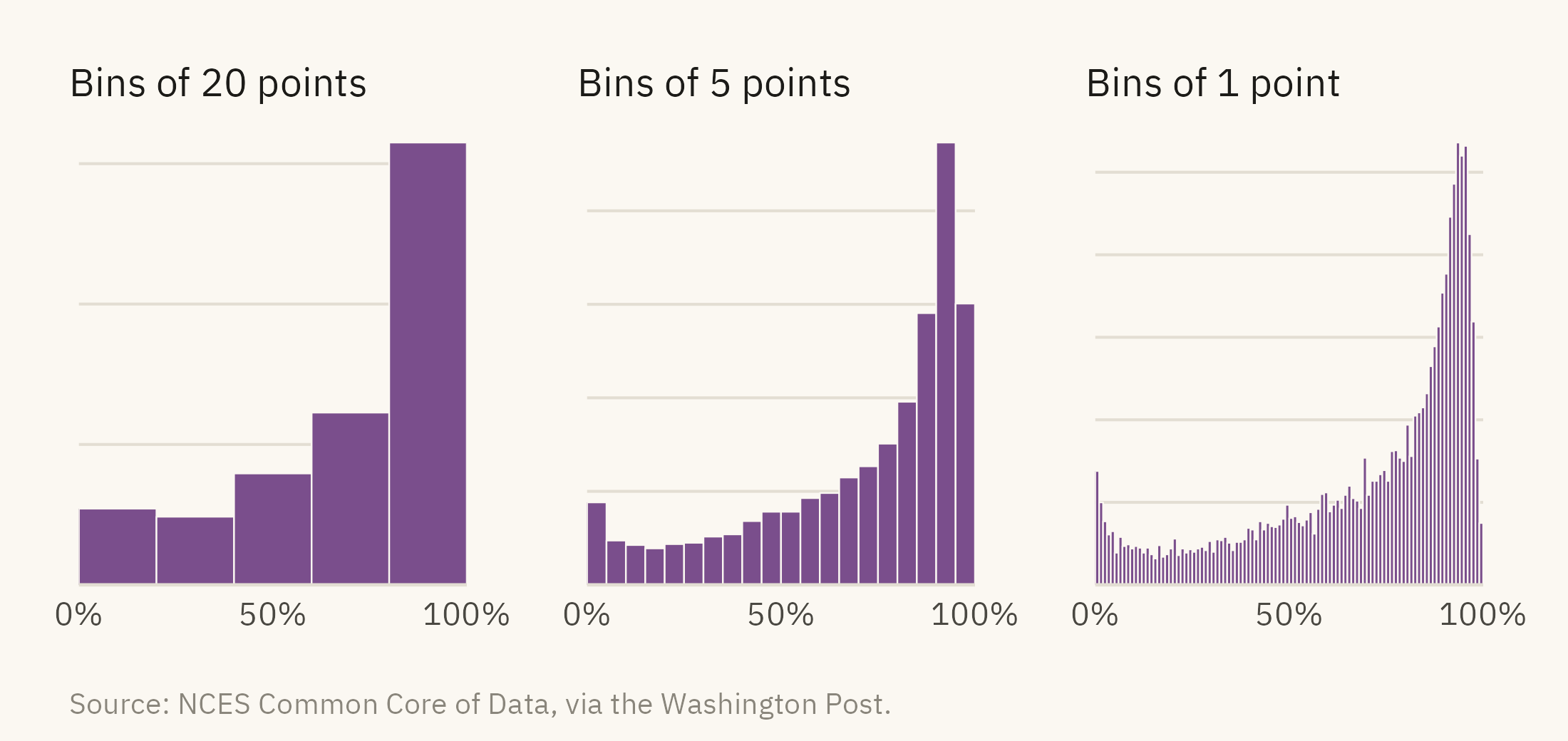
A histogram has one setting, the bin width. The bin width changes the shape that appears in the chart. Figure 5.2 draws the same data three ways.
Show the code
bins <-function(bw, title) {ggplot(d17, aes(white)) +geom_histogram(binwidth = bw, boundary =0, fill =mv_accent(), color = mv_ink$canvas, linewidth =0.2) +scale_x_continuous(labels =label_percent(scale =1), breaks =c(0, 50, 100), expand =expansion(0)) +scale_y_continuous(expand =expansion(mult =c(0, 0.05))) +labs(x =NULL, y =NULL, title = title) +theme_mv(base_size =10) + plain_title +theme(axis.text.y =element_blank())}bins(20, "Bins of 20 points") +bins(5, "Bins of 5 points") +bins(1, "Bins of 1 point") +plot_annotation(caption =mv_source(src), theme = cap_theme)
Figure 5.2: The same distribution with bins of 20, 5, and 1 percentage point. The wide bins leave out the shape. The narrow bins are jagged, and neighboring bars differ by chance. The middle panel shows the shape with the least noise. Source: NCES Common Core of Data, via the Washington Post.
There is no single correct bin width. The usual practice is to try several and publish the one that shows the shape with the least noise. The caption should state the bin width used. With a bin width of 20, the left panel has five bars. With a bin width of 1, the bars below 50 percent hold a few dozen districts each, and bars next to each other differ by chance. The right panel is jagged, and the jaggedness is noise, not shape. The bars at 93 to 96 percent hold more than 500 districts each. The bar at 99 to 100 percent holds 75. With a bin width of 5, those differences are averaged out and the shape is smooth. Chapter 9 returns to the question of when a detail is worth including.
5.3 Skew and the Log Scale
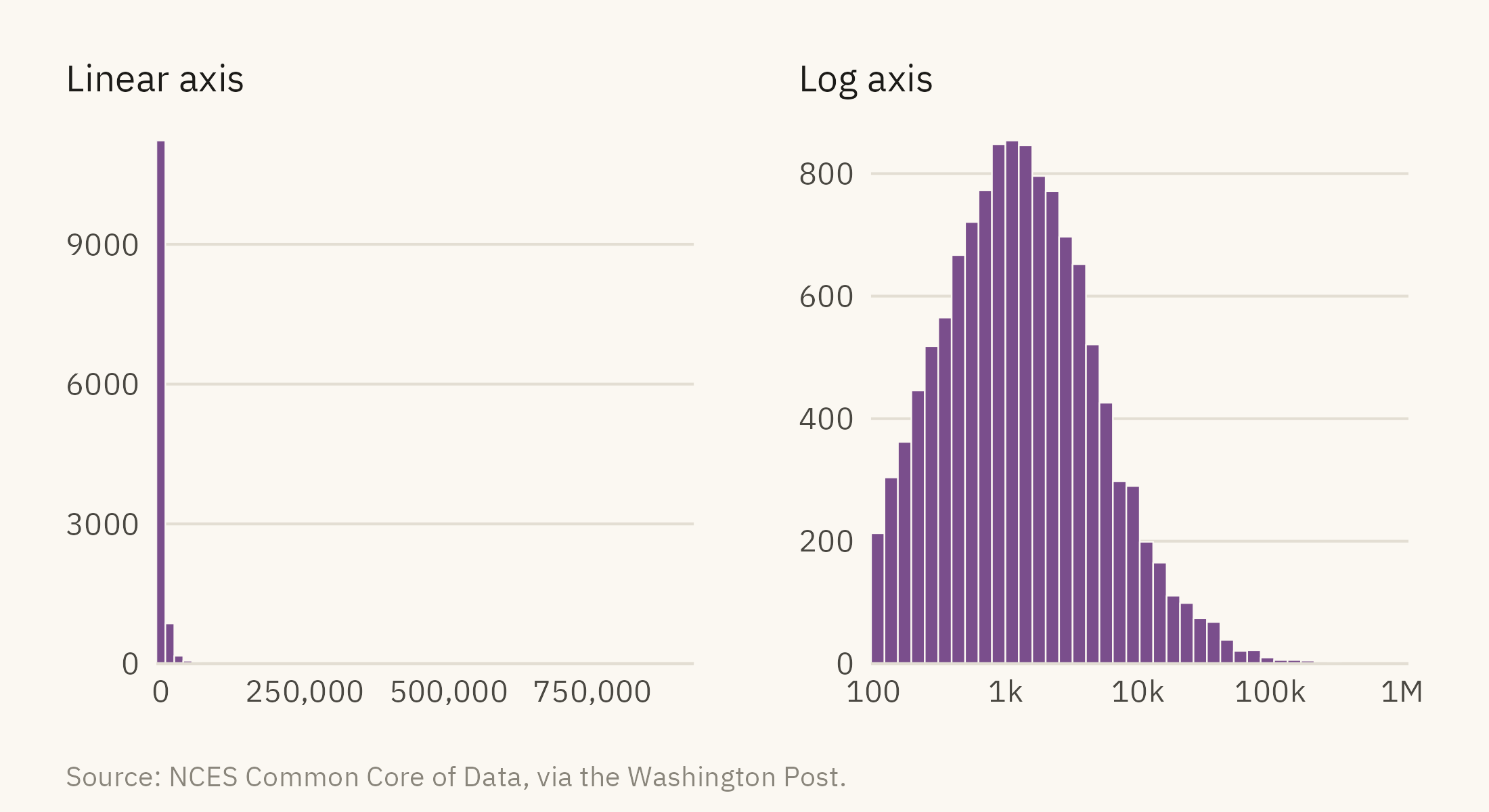
Enrollment is the other variable in the data. Its shape is hard to see on a linear axis. Figure 5.3 draws it twice.
Show the code
lin <-ggplot(d17, aes(enrollment)) +geom_histogram(bins =60, fill =mv_accent(), color = mv_ink$canvas, linewidth =0.2) +scale_x_continuous(labels =label_comma(), expand =expansion(0)) +scale_y_continuous(expand =expansion(mult =c(0, 0.05))) +labs(x =NULL, y =NULL, title ="Linear axis") +theme_mv(base_size =10) + plain_titlelg <-ggplot(d17, aes(enrollment)) +geom_histogram(bins =40, fill =mv_accent(), color = mv_ink$canvas, linewidth =0.2) +scale_x_log10(labels =c("100", "1k", "10k", "100k", "1M"), breaks =c(100, 1000, 10000, 100000, 1e6), expand =expansion(0)) +scale_y_continuous(expand =expansion(mult =c(0, 0.05))) +labs(x =NULL, y =NULL, title ="Log axis") +theme_mv(base_size =10) + plain_titlelin + lg +plot_annotation(caption =mv_source(src), theme = cap_theme)
Figure 5.3: District enrollment, 2016-17. Left, on a linear axis, nearly every district falls in the first bar, and the axis extends past 900,000 because of New York City. Right, on a log axis, the distribution is bell-shaped and centered near 1,200 students. The largest districts form a thin tail on the right. Source: NCES Common Core of Data, via the Washington Post.
A log scale spaces values by ratio rather than by difference. Each tick is ten times the one before. A log axis is suitable for a variable that spans several orders of magnitude, such as population, income, or firm size. For a variable that spans less than one order of magnitude, a linear axis is usually the better choice. The tick labels and the caption should both state that the axis is a log scale. A reader who misses that may assume the bell-shaped distribution refers to equal intervals of enrollment.
5.4 Several Groups: Boxes, Violins, and Dots
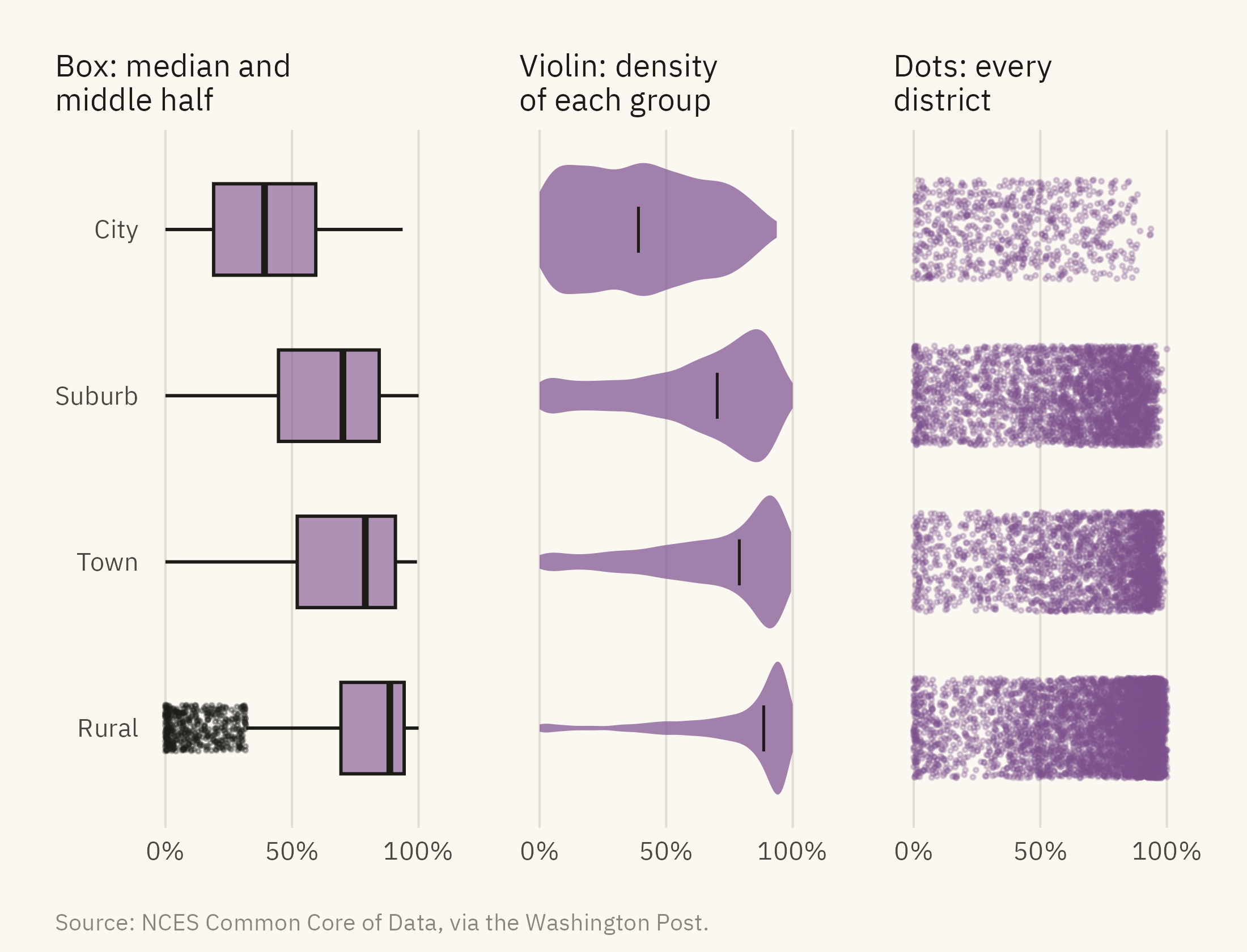
A histogram shows one variable. The next question is how the distribution differs across groups. The locale of each district (city, suburb, town, or rural) is one grouping in the data. Figure 5.4 shows three ways to compare the four locales.
Figure 5.4: Share of white students by district locale, 2016-17, drawn three ways. The box plot shows the median and middle half. The violin shows the full shape, including the pile-up of rural districts near 100 percent. The dots show every district and how many there are in each group. Source: NCES Common Core of Data, via the Washington Post.
The box plot summarizes a distribution with five numbers. The line in the box is the median. The box is the middle half of the data, from the 25th to the 75th percentile. The whiskers extend to the furthest values within one and a half box widths. Values beyond the whiskers are drawn as points. The box plot is compact, and it leaves out the shape of the distribution. The rural box shows that the median is 89 and the middle half runs from 69 to 94. It does not show the concentration of districts at 100.
The violin shows that concentration. It draws the density of each group as a shape, mirrored for symmetry. The rural violin is wide at the right end, near 100 percent, and thin everywhere else. The city violin is wide across the whole range, which means city districts vary more than districts in any other locale. Violins take more space than boxes. They also need enough data to estimate a density, a few dozen values at least.
The dot panel shows the number of districts in each group, which neither summary shows. There are 6,200 rural districts and 730 city districts. The rural cloud is dense and the city cloud is sparse. A reader can see which group makes up most of the national figures. When groups differ in size, the chart should show the dots or print the counts.
5.5 Many Groups: Ridgelines
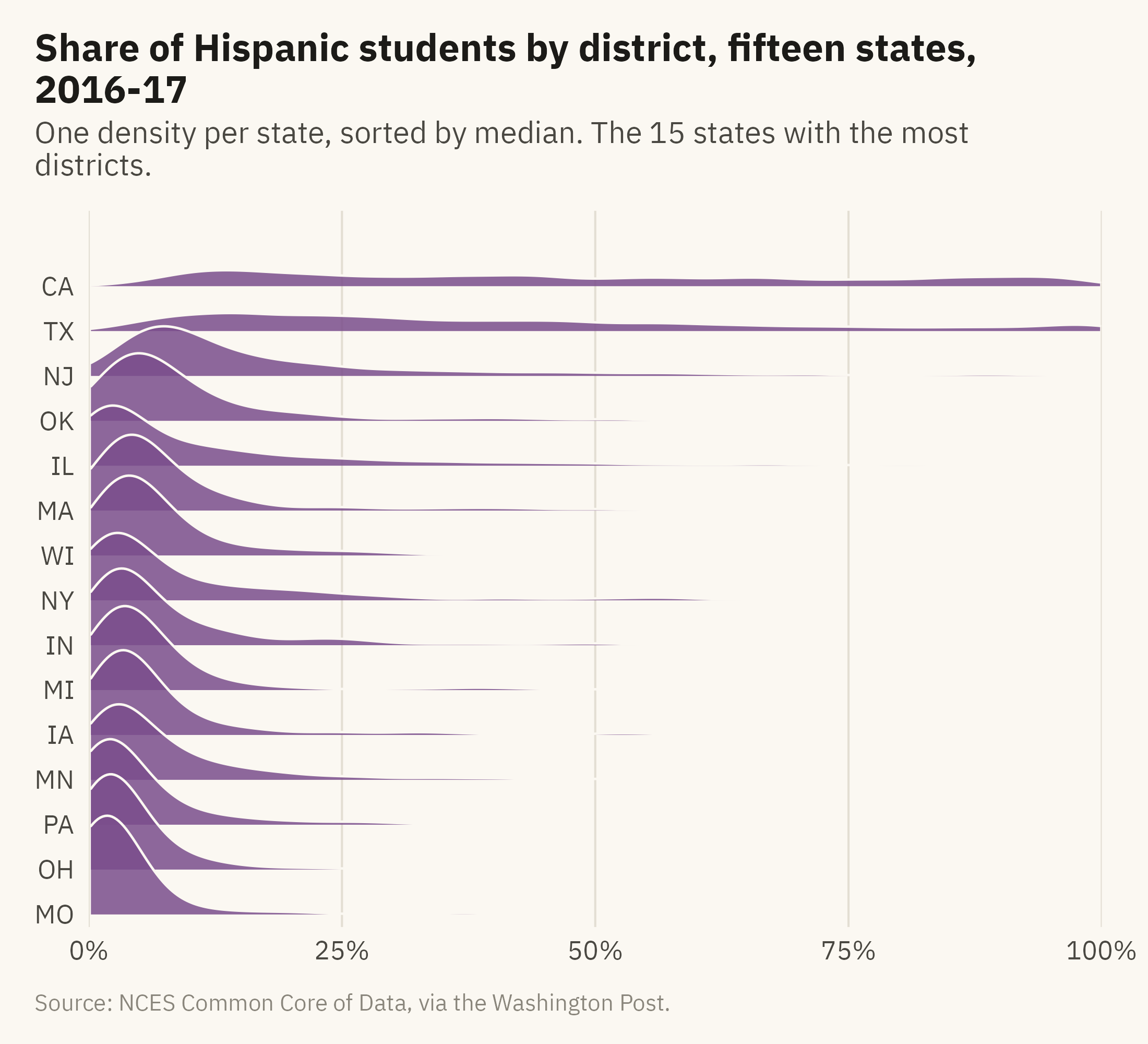
Four groups fit side by side in Figure 5.4. Fifteen groups would not fit in that layout. The ridgeline plot stacks one density per group with a small overlap. Twenty distributions can fit in the space of five. Figure 5.5 shows the share of Hispanic students by district for the fifteen states with the most districts.
Show the code
states15 <- d17 |>count(state) |>slice_max(n, n =15) |>pull(state)rd <- d17 |>filter(state %in% states15) |>mutate(state =fct_reorder(state, hispanic, .fun = median))ggplot(rd, aes(hispanic, state)) +geom_density_ridges(fill =mv_accent(), color = mv_ink$canvas, alpha =0.85, scale =2.2,rel_min_height =0.005, bandwidth =3, linewidth =0.4) +scale_x_continuous(labels =label_percent(scale =1), limits =c(0, 100), expand =expansion(0)) +scale_y_discrete(expand =expansion(mult =c(0.02, 0.12))) +labs(title ="Share of Hispanic students by district, fifteen states, 2016-17",subtitle ="One density per state, sorted by median. The 15 states with the most districts.",x =NULL, y =NULL, caption =mv_source(src)) +theme_mv(grid ="x")
Figure 5.5: Share of Hispanic students by district in the fifteen states with the most districts, 2016-17, each drawn as a density and sorted by median. California and Texas have broad distributions reaching past 80 percent. New Jersey has a long tail. In the other twelve states, nearly every district is below 20 percent. Source: NCES Common Core of Data, via the Washington Post.
A ridgeline plot shows many groups at the cost of precision. A reader cannot read a percentile from a ridge, and the overlap covers the tail of the ridge below. A reader can compare fifteen shapes at once and see which states differ. The order of the groups affects what a reader can see. Sorted by median, as in Figure 5.5, the shapes change gradually from bottom to top. Sorted alphabetically, the same ridges would show no progression.
5.6 Comparing Two Distributions: The Cumulative Curve
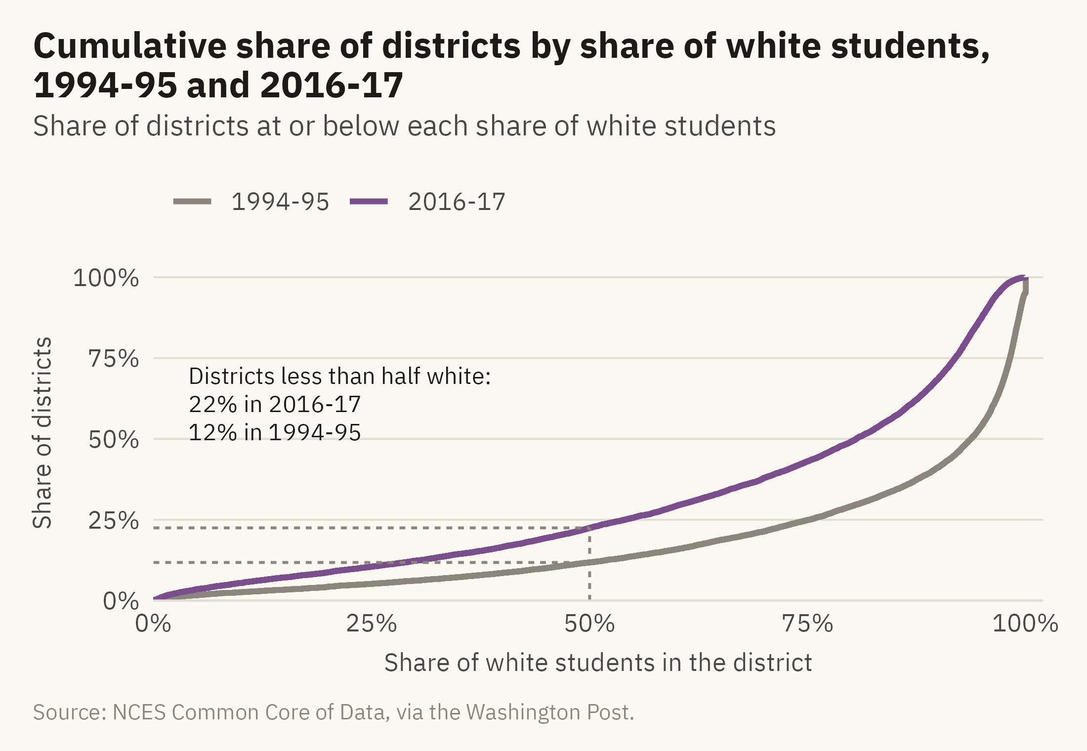
The data contains two school years, 1994-95 and 2016-17. The question is how the distribution changed between them. Two histograms side by side require the reader to compare shapes. Two overlaid histograms cover each other. A third option is the cumulative distribution. For each value on the horizontal axis, it draws the share of districts at or below that value. Figure 5.6 shows the two years.
Show the code
ec <- d |>mutate(year =factor(year, labels =c("1994-95", "2016-17")))ggplot(ec, aes(white, color = year)) +stat_ecdf(linewidth =1, pad =FALSE) +annotate("segment", x =50, xend =50, y =0, yend =0.225, color = mv_ink$mute, linewidth =0.5, linetype ="22") +annotate("segment", x =0, xend =50, y =0.118, yend =0.118, color = mv_ink$mute, linewidth =0.5, linetype ="22") +annotate("segment", x =0, xend =50, y =0.225, yend =0.225, color = mv_ink$mute, linewidth =0.5, linetype ="22") +annotate("text", x =4, y =0.72, label ="Districts less than half white:\n22% in 2016-17\n12% in 1994-95",hjust =0, vjust =1, size =3, family =mv_font(), color = mv_ink$ink, lineheight =1) +scale_color_manual(values =c(`1994-95`= mv_ink$mute, `2016-17`=mv_accent()), name =NULL) +scale_x_continuous(labels =label_percent(scale =1), expand =expansion(mult =c(0, 0.02))) +scale_y_continuous(labels =label_percent(), expand =expansion(mult =c(0, 0.04))) +labs(title ="Cumulative share of districts by share of white students, 1994-95 and 2016-17",subtitle ="Share of districts at or below each share of white students",x ="Share of white students in the district", y ="Share of districts",caption =mv_source(src)) +theme_mv()
Figure 5.6: Cumulative share of districts by share of white students, 1994-95 and 2016-17. Read a value on the horizontal axis up to the curve to find the share of districts at or below it. The 2016-17 curve is above the earlier one at every point, which means more districts at every level of diversity. In 1994-95, 12 percent of districts were less than half white. In 2016-17, 22 percent were. The 1994-95 curve rises by 5 points at the right edge, where 642 districts reported no students of color. Source: NCES Common Core of Data, via the Washington Post.
The cumulative curve has three advantages for comparing distributions. It needs no bins, so there is no bin width to choose. It shows every percentile at once. Two curves can be overlaid without covering each other. The disadvantage is that many readers have not seen one before and need a sentence of instruction. The caption and the annotations in Figure 5.6 supply those instructions. Once a reader knows that the curve on top has more districts below any given value, the same reading applies to any pair of distributions.
5.7 The Edges
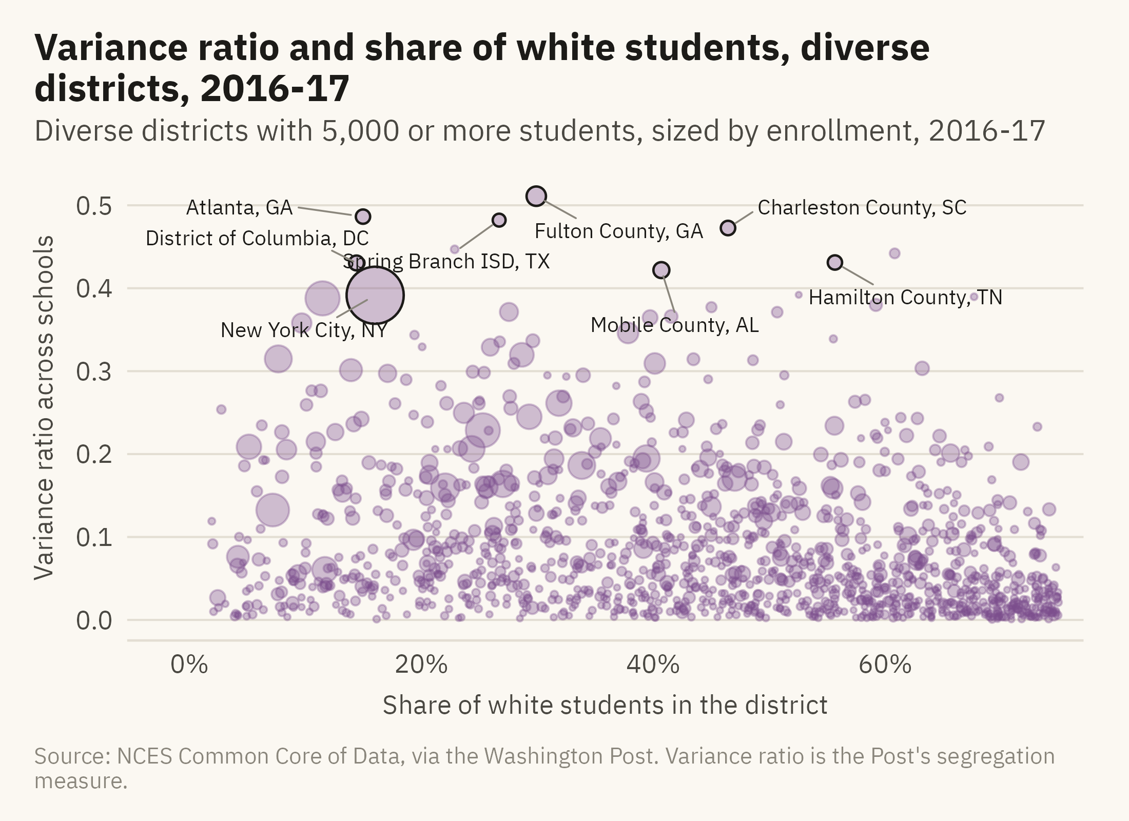
The last question is which districts are at the edges. For that question, individual districts need to be named. The Post’s data includes a measure of how evenly each district spreads its students across its own schools. The Post calls it the variance ratio. A district can be diverse as a whole and segregated school by school. Figure 5.7 shows those districts.
Show the code
edges <- d17 |>filter(diversity =="Diverse", !is.na(variance_ratio), enrollment >=5000)named <- edges |>filter(enrollment >=30000) |>slice_max(variance_ratio, n =8) |>mutate(district =str_replace(district, " (Public Schools|School District|Independent School District|Schools|County Public Schools|Unified)$", ""),district =str_replace(district, " Isd$", " ISD"),district =str_replace(district, "^District Of Columbia$", "District of Columbia"),district =str_replace(district, "^Charleston 01$", "Charleston County"),district =paste0(district, ", ", state))ggplot(edges, aes(white, variance_ratio)) +geom_point(aes(size = enrollment), color =mv_accent(), alpha =0.35) +geom_point(data = named, aes(size = enrollment), color = mv_ink$ink, shape =21, stroke =0.6, fill =NA) +geom_text_repel(data =filter(named, state !="DC"), aes(label = district), size =2.6, family =mv_font(), color = mv_ink$ink,min.segment.length =0, segment.color = mv_ink$mute, segment.size =0.3, box.padding =0.6,point.padding =0.4, force =3, seed =5, max.overlaps =20) +geom_text_repel(data =filter(named, state =="DC"), aes(label = district), size =2.6, family =mv_font(), color = mv_ink$ink,min.segment.length =0, segment.color = mv_ink$mute, segment.size =0.3,nudge_x =-11, nudge_y =0.03, hjust =1, seed =5) +scale_size_area(max_size =9, guide ="none") +scale_x_continuous(labels =label_percent(scale =1), expand =expansion(mult =c(0.1, 0.03))) +labs(title ="Variance ratio and share of white students, diverse districts, 2016-17",subtitle ="Diverse districts with 5,000 or more students, sized by enrollment, 2016-17",x ="Share of white students in the district", y ="Variance ratio across schools",caption =mv_source(src, "Variance ratio is the Post's segregation measure")) +theme_mv()
Figure 5.7: Districts classified as diverse in 2016-17, by the share of their students who are white and the variance ratio across their schools. A high ratio means students of different groups attend different schools within the same district. Named: the eight highest variance ratios among districts with 30,000 or more students. Source: NCES Common Core of Data, via the Washington Post.
The other charts in this chapter do not name individual districts. Figure 5.7 names eight. At the edges, a reader usually wants to know which districts are there. A point far from the others with no label does not answer that question. When outliers are labeled, the caption should state the rule used to choose them.
ImportantEthics Moment: The Unit of Analysis
Every chart in this chapter counts districts. A district of 140 students and a district of a million are each one dot, one row, or one slice of a density. Rural districts are most of the districts and enroll a small share of the students, so they determine most of each shape in the chapter. The student-weighted mean in Figure 5.1 is the only place where a chart counts students rather than administrative units.
Either choice can be correct. A chart about how districts are governed should count districts. A chart about what students experience should count students. A chart that does not state which unit it counts leaves the reader to assume one. In this subject, the two units lead to opposite conclusions about how segregated American schools are.
TipTry It Online
Shape of a Variable at viz.marginoferrormedia.com/apps contains the district data. Pick a variable, a grouping, and a chart. Drag the bin width to see the histogram change. A toggle switches every chart from counting districts to counting students. Note what the switch does to the rural ridge.
WarningAI Reality Check: The Summary Is Not the Shape
Ask a model to describe the share of white students across districts. It will usually report a mean of 70, a median of 80, and perhaps a standard deviation. Those numbers are correct. None of them shows the concentration at 100 and the long tail to zero. None of them shows that few districts are near the mean. Chapter 1 made this point with Anscombe’s Quartet. In the district data, the summary leaves out the shape and also gives a misleading picture of the typical district.
The correction is the same as in Chapter 1. Ask for the histogram before the mean. When a model reports a mean, ask which unit it averaged. The district average and the student average are about twenty points apart. The model will often have chosen one without saying so.
5.8 Putting It All Together
A distribution answers three questions that a single number cannot. What is typical, how much the values vary, and which cases are at the edges. The histogram is the first chart to draw, and the bin width is its one setting. Skewed variables need a log axis, labeled as such. Groups can be compared with boxes when space is short, violins when shape matters, dots when group sizes differ, and ridgelines when there are many groups. Two distributions can be compared as cumulative curves. The cases at the edges should be labeled. Every chart in the chapter depends on the choice of unit, districts or students, and that choice determines what the shapes mean.
5.9 Looking Ahead
Chapter 6 adds a second variable. The question is whether two variables move together, and the scatter plot is the chart for that question. The case is what people study and what they earn. The two are related, and there are many exceptions. The chapter also explains why a relationship in a scatter plot does not show cause.
5.10 Further Reading and References
Cleveland, W. S. (1993). Visualizing Data. Hobart Press. The source for most of the distribution displays here, including the quantile plot, which the cumulative curve is based on.
Meckler, L., and Rabinowitz, K. (2019). How the nation’s growing racial diversity is changing our schools. The Washington Post, September 12. The analysis the data in this chapter comes from, with the definitions of diverse and integrated used here.
Tukey, J. W. (1977). Exploratory Data Analysis. Addison-Wesley. The box plot’s origin and the argument for looking at the data before summarizing it.
Wilke, C. O. (2019). Fundamentals of Data Visualization. O’Reilly. Chapters 7 through 9 cover distributions, including ridgelines and cumulative curves.
Wilkinson, L. (1999). Dot plots. The American Statistician, 53(3), 276–281. The dot display for small and medium data, and its history.
5.11 Key Terms
Histogram. Values sorted into bins, a bar per bin, height equal to the count. The bin width is a choice.
Log scale. An axis spaced by ratio, where each tick is a multiple of the last. For variables spanning orders of magnitude.
Box plot. The median, the middle half, the whiskers, and the outliers. Compact, and it leaves out the shape of the distribution.
Violin. A mirrored density per group. It shows shape and needs a few dozen values per group.
Ridgeline. Stacked densities with overlap, for many groups.
Cumulative distribution. For each value, the share of observations at or below it. Compares distributions without bins.
Unit of analysis. What one row represents. A district or a student. The choice changes every chart.
5.12 Exercises
Check Your Understanding
The mean share of white students is 70 and the median is 80. Using Figure 5.1, explain in one sentence why the mean is below the median.
In the one-point histogram, the bars at 93 to 96 percent hold more than 500 districts each and the bar at 99 to 100 holds 75. Explain why neighboring bars differ by chance when bins are narrow, and why the five-point histogram is smoother.
State the five numbers a box plot shows. Which feature does the rural box in Figure 5.4 leave out, and which chart shows it?
In Figure 5.6, how would you read off the share of districts that were at least 90 percent white in each year?
Why does Figure 5.3 need to state that its right panel is on a log scale?
Apply It
Using ch05-school-districts.csv, draw a histogram of the share of Black students in 2016-17. Choose and justify a bin width. Describe the shape in two sentences.
Draw box plots of enrollment by locale on a log axis. Which locale has the widest middle half?
Build the ridgeline in Figure 5.5 for the share of Black students instead. Which states move to the top?
Compute the student-weighted mean share of white students by locale and compare it with the district mean in each. Where is the gap largest, and what does that say about those districts?
Think Deeper
The chapter says most readers have not seen a cumulative curve before. Write a two-sentence caption that would tell a first-time reader how to read Figure 5.6 without the annotations.
A policy brief reports that “the typical district is 80 percent white.” Write a reply that explains, using the unit of analysis, why a parent might not recognize that description.
Figure 5.7 labels eight districts and leaves hundreds unlabeled. Propose a rule for which points on a scatter plot should get a name, and apply it to the chart.