6  Relationship

6.1 What You Study and What You Earn

The American Community Survey asks a million people a year what they studied in college and what they earn. FiveThirtyEight compiled the answers for recent graduates in 172 majors. Earnings differ widely by major. Petroleum engineers earn a median of $110,000 a few years out of school. Library science graduates earn $22,000. Among the facts known about a recent graduate, the major is one of the strongest predictors of earnings (Carnevale, Cheah, and Hanson, 2015).

Earnings is one variable. This chapter is about two variables at once. The questions are whether two measures move together, how they move together, and whether the pattern holds inside subgroups. The second variable here is the share of each major’s graduates who are women. The relationship between the two has been studied in the economics of education (Levanon, England, and Allison, 2009). Majors with more women tend to pay less. The scatter plot is the chart for two numeric variables. The rest of the chapter describes what a scatter plot shows and what it leaves out.

6.2 The Scatter Plot

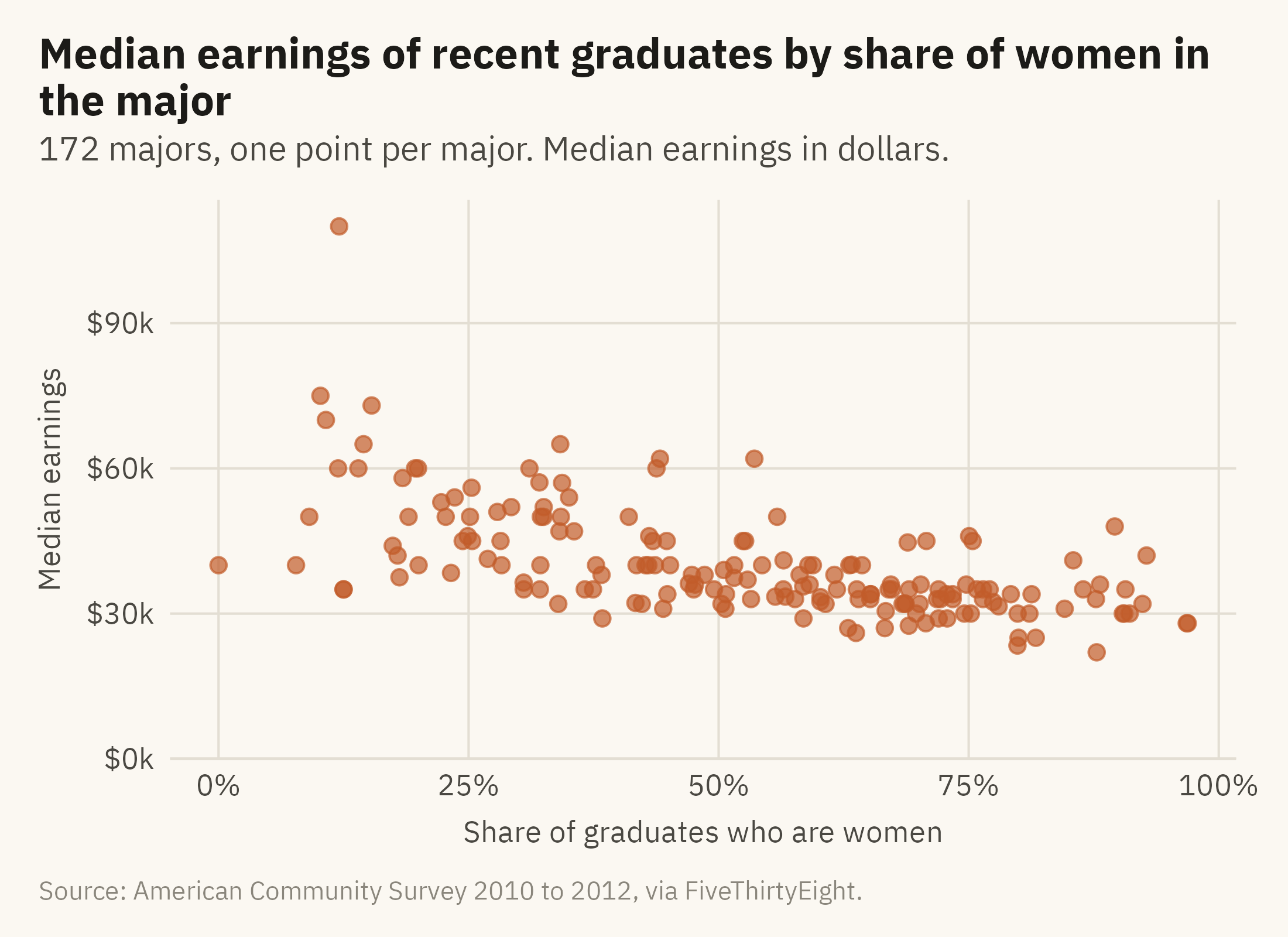
A scatter plot puts one variable on each axis and one point per observation. It uses position on two common scales, which is the highest encoding on the hierarchy from Chapter 2. Every observation is drawn, so the relationship can be seen before any summary is computed. Figure 6.1 shows the 172 majors.

ggplot(m, aes(share_women, median)) +
  geom_point(color = mv_accent(), size = 2, alpha = 0.7) +
  scale_x_continuous(labels = label_percent()) +
  scale_y_continuous(labels = label_dollar(scale = 1e-3, suffix = "k"), limits = c(0, NA), expand = expansion(mult = c(0, 0.05))) +
  labs(title = "Median earnings of recent graduates by share of women in the major",
       subtitle = "172 majors, one point per major. Median earnings in dollars.",
       x = "Share of graduates who are women", y = "Median earnings",
       caption = mv_source(src)) +
  theme_mv(grid = "y") +
  theme(panel.grid.major.x = element_line(color = mv_ink$grid, linewidth = 0.35))

Figure 6.1: Median earnings of recent graduates against the share of women among graduates, one point per major. The relationship is negative and loose. The correlation is -0.62. Source: American Community Survey 2010 to 2012, via FiveThirtyEight.

Three features of a scatter plot can be read in order. Direction comes first. The cloud slopes down to the right, so majors with a higher share of women tend to have lower earnings. Strength comes second. The cloud is wide. Near 50 percent women, median earnings range from $31,000 to $62,000. A correlation of -0.62 is a moderate relationship. Much of the variation in earnings is not explained by the share of women. Shape comes third. The cloud is roughly a band rather than a curve. It is thinner at the right than at the left. One point is separate from the rest at the top. Most scatter plots contain a few points that readers will want identified, and these should be labeled, as in Figure 6.3.

6.3 Fitting a Line

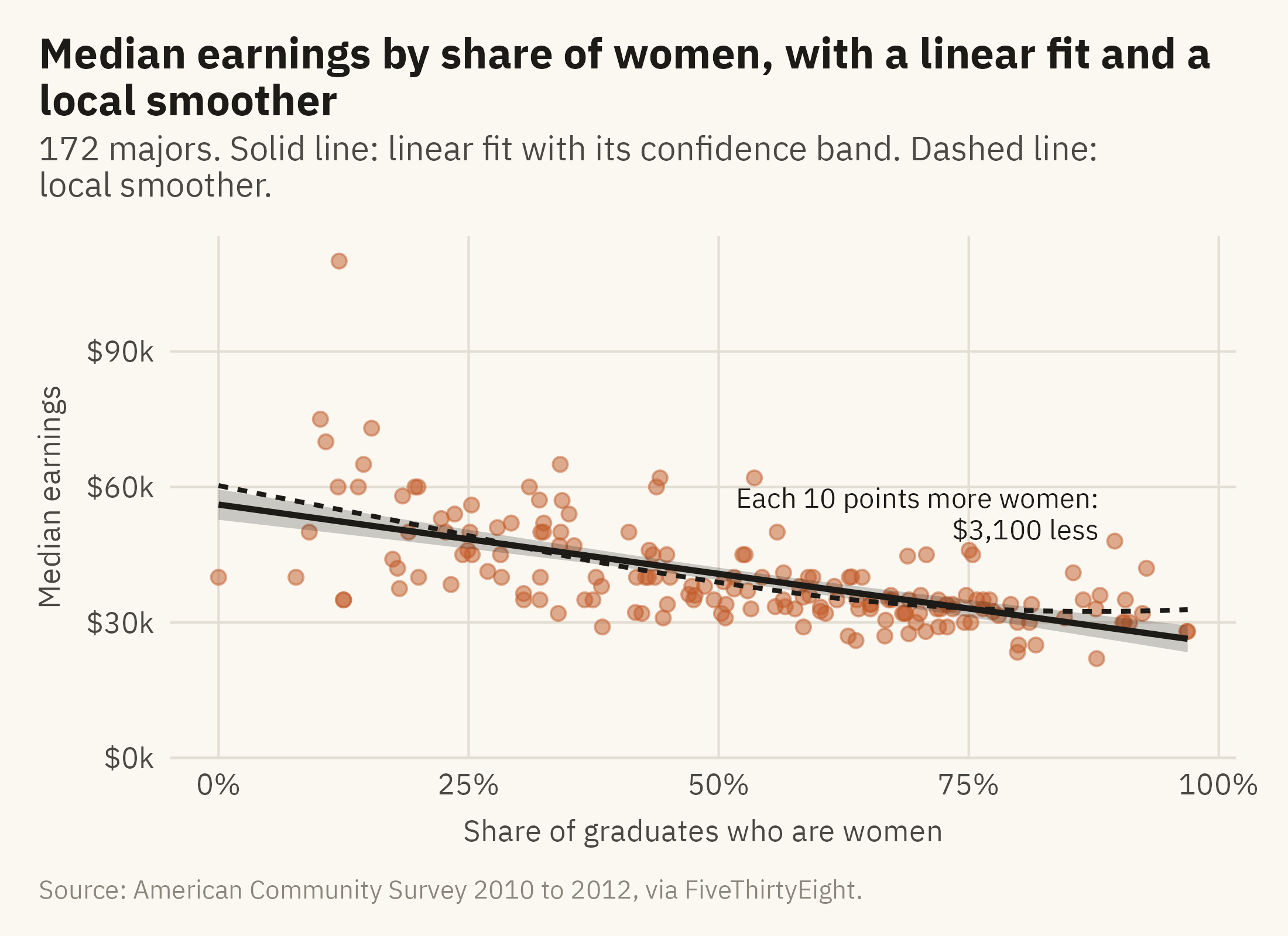
A fitted line summarizes the direction of a relationship as a slope. Figure 6.2 adds two lines. One is the least-squares line, which is the standard summary. The other is a local smoother, which follows the points without assuming a straight line.

slope <- coef(lm(median ~ share_women, m))[2]
ggplot(m, aes(share_women, median)) +
  geom_point(color = mv_accent(), size = 1.8, alpha = 0.5) +
  geom_smooth(method = "loess", se = FALSE, color = mv_ink$ink, linewidth = 0.7, linetype = "22", formula = y ~ x, span = 0.9) +
  geom_smooth(method = "lm", color = mv_ink$ink, fill = mv_ink$ink, alpha = 0.22, linewidth = 0.9, formula = y ~ x) +
  annotate("text", x = 0.88, y = 54000, label = paste0("Each 10 points more women:\n", label_dollar()(round(-slope / 10, -2)), " less"),
           hjust = 1, size = 3, family = mv_font(), color = mv_ink$ink, lineheight = 0.95) +
  scale_x_continuous(labels = label_percent()) +
  scale_y_continuous(labels = label_dollar(scale = 1e-3, suffix = "k"), limits = c(0, NA), expand = expansion(mult = c(0, 0.05))) +
  labs(title = "Median earnings by share of women, with a linear fit and a local smoother",
       subtitle = "172 majors. Solid line: linear fit with its confidence band. Dashed line: local smoother.",
       x = "Share of graduates who are women", y = "Median earnings", caption = mv_source(src)) +
  theme_mv(grid = "y") +
  theme(panel.grid.major.x = element_line(color = mv_ink$grid, linewidth = 0.35))

Figure 6.2: The same points with a straight-line fit (solid) and a local smoother (dashed). The slope of the line means that a major with ten points more women pays about $3,100 less. The smoother follows the line across most of the range and flattens at the right. The band around the line shows the uncertainty in the line, not the spread of the points. Source: American Community Survey 2010 to 2012, via FiveThirtyEight.

Two cautions apply to fitted lines. First, a line is a summary of the points and should be drawn with them. Anscombe’s four datasets in Chapter 1 have the same fitted line and different shapes. When the line is drawn without the points, those differences cannot be seen. Secondly, the shaded band is a confidence band for the line. It shows the range within which the fitted line would fall under repeated sampling, and it narrows as the number of points grows. It does not show the spread of the points. A reader who takes the band for the spread of majors will overstate how tight the relationship is.

6.4 Who Is Where: Labels and Size

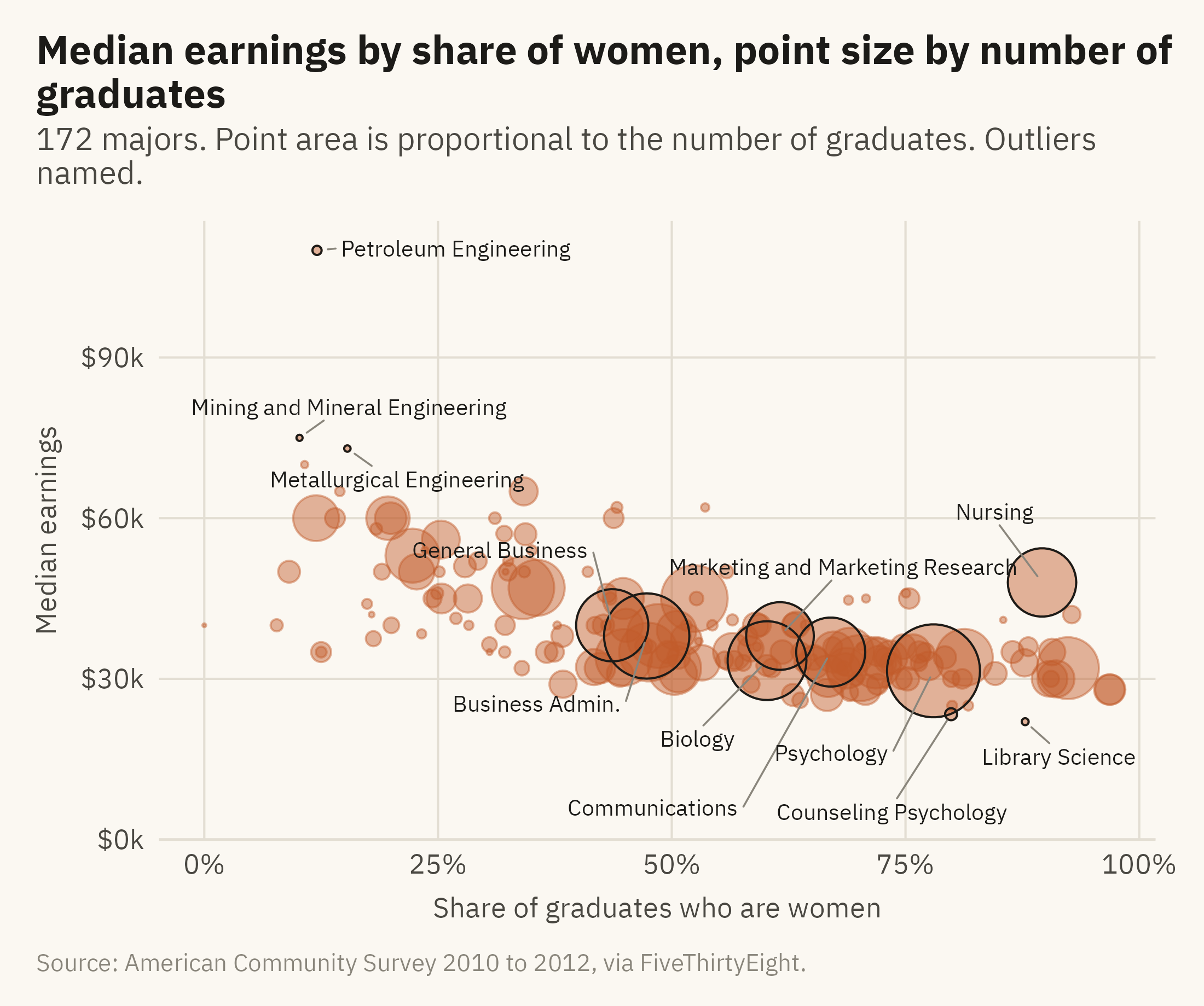
The point at the top of Figure 6.1 is petroleum engineering. A reader should be able to learn that from the chart itself. Figure 6.3 names the points that are furthest from the rest. It also sizes each point by the number of graduates.

named <- m |> filter(median >= 73000 | median <= 23500 | graduates >= 200000) |>
  mutate(major = str_replace(major, "Business Management and Administration", "Business Admin."),
         ny = case_when(major %in% c("General Business", "Marketing and Marketing Research") ~ 14000,
                        major %in% c("Business Admin.", "Biology", "Communications") ~ -14000,
                        major == "Psychology" ~ -16000,
                        major == "Counseling Psychology" ~ -12000,
                        major == "Library Science" ~ -9000,
                        major == "Nursing" ~ 12000,
                        TRUE ~ 0),
         nx = case_when(major == "General Business" ~ -0.12, major == "Business Admin." ~ -0.1,
                        major == "Marketing and Marketing Research" ~ 0.08,
                        major == "Biology" ~ -0.08, major == "Communications" ~ 0.04,
                        major == "Psychology" ~ -0.12, major == "Counseling Psychology" ~ -0.02,
                        major == "Library Science" ~ 0.03, major == "Nursing" ~ -0.06,
                        TRUE ~ 0))
ggplot(m, aes(share_women, median)) +
  geom_point(aes(size = graduates), color = mv_accent(), alpha = 0.45) +
  geom_point(data = named, aes(size = graduates), color = mv_ink$ink, shape = 21, stroke = 0.5, fill = NA) +
  geom_text_repel(data = named, aes(label = major), size = 2.6, family = mv_font(), color = mv_ink$ink,
                  nudge_x = named$nx, nudge_y = named$ny,
                  min.segment.length = 0, segment.color = mv_ink$mute, segment.size = 0.3,
                  box.padding = 0.45, point.padding = 0.3, max.overlaps = 30, seed = 6) +
  scale_size_area(max_size = 14, guide = "none") +
  scale_x_continuous(labels = label_percent()) +
  scale_y_continuous(labels = label_dollar(scale = 1e-3, suffix = "k"), limits = c(0, NA), expand = expansion(mult = c(0, 0.05))) +
  labs(title = "Median earnings by share of women, point size by number of graduates",
       subtitle = "172 majors. Point area is proportional to the number of graduates. Outliers named.",
       x = "Share of graduates who are women", y = "Median earnings", caption = mv_source(src)) +
  theme_mv(grid = "y") +
  theme(panel.grid.major.x = element_line(color = mv_ink$grid, linewidth = 0.35))

Figure 6.3: The same relationship with each major sized by its number of graduates. Named: the three highest and two lowest medians, and the seven majors with more than 200,000 graduates. Petroleum engineering, with 2,300 graduates, is alone at the top. Psychology, with 393,000, is among the many majors at the lower right. The three largest majors are psychology, business administration, and biology. Source: American Community Survey 2010 to 2012, via FiveThirtyEight.

Size adds a third variable to a scatter plot. Area is low on the hierarchy, so a reader can tell large from small but cannot judge the ratio between two points. For this chart that is sufficient, because the number of graduates is context rather than the main comparison. The chart shows that the high-paying majors at the upper left have few graduates. Most graduates are in majors at the lower right. Nursing, at 90 percent women and $48,000, is the large point above the trend. A fitted line alone would not show this exception.

Labels are placed on the points a reader is most likely to ask about. These are usually the extremes, the largest, and the ones that depart from the pattern. The caption states the rule that selected them. Labeling all 172 majors would make the chart too crowded to read.

6.5 Inside the Relationship: Small Multiples

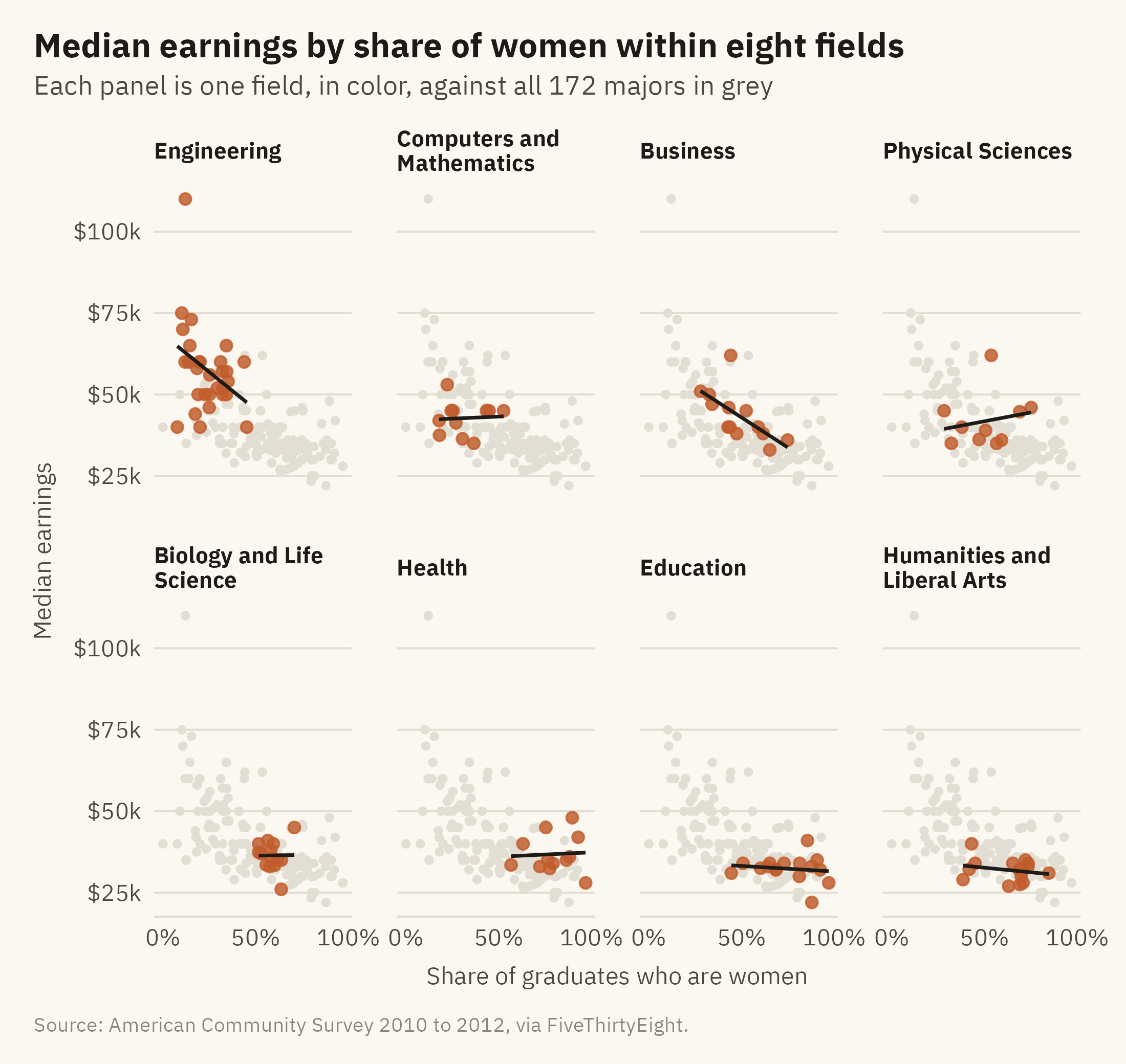
The charts so far treat the 172 majors as one population. The majors fall into fields, and the fields differ on both variables. Engineering majors are mostly men and are mostly well paid. Education majors are mostly women and are mostly paid less. Part of the overall slope comes from the difference between fields rather than from a relationship within any field. Figure 6.4 draws the scatter plot inside each of the eight largest fields.

cats <- m |> count(category) |> filter(n >= 10) |> pull(category)
fm <- m |> filter(category %in% cats) |>
  mutate(category = str_replace(category, " & ", " and "),
         category = fct_reorder(category, median, .fun = stats::median, .desc = TRUE))
ggplot(fm, aes(share_women, median)) +
  geom_point(data = select(m, -category), color = mv_ink$grid, size = 0.9) +
  geom_point(color = mv_accent(), size = 1.6, alpha = 0.8) +
  geom_smooth(method = "lm", se = FALSE, color = mv_ink$ink, linewidth = 0.6, formula = y ~ x) +
  facet_wrap(~ category, ncol = 4, labeller = label_wrap_gen(22)) +
  scale_x_continuous(labels = label_percent(), breaks = c(0, 0.5, 1)) +
  scale_y_continuous(labels = label_dollar(scale = 1e-3, suffix = "k"), breaks = c(25000, 50000, 75000, 100000)) +
  labs(title = "Median earnings by share of women within eight fields",
       subtitle = "Each panel is one field, in color, against all 172 majors in grey",
       x = "Share of graduates who are women", y = "Median earnings", caption = mv_source(src)) +
  theme_mv(base_size = 10) +
  theme(strip.text = element_text(size = rel(0.8)))

Figure 6.4: Median earnings by share of women within each of eight fields, with a fitted line per field, all on the same axes. The slope is steep within engineering and business, shallow within education and humanities, and flat within computing, biology, and health. Part of the overall pattern is between fields and part is within them. Source: American Community Survey 2010 to 2012, via FiveThirtyEight.

The grey points are the full dataset, repeated in every panel as a reference. Without the reference, a reader cannot tell whether a field is high or low compared with the others.

The panels show the relationship within each field. Within engineering, majors with more women pay less, and the slope is steep. Within computing, the share of women is unrelated to pay. Within health, nursing raises the fitted line. When a relationship appears in the whole and weakens in the parts, a third variable is often involved. Here that variable is the field.

6.6 Correlation Is Not a Direction

A reader of Figure 6.2 may want to write a sentence like “majors that admit more women pay less.” The data do not support that sentence. The scatter plot shows that two variables move together. It does not show which one affects the other, or whether a third variable affects both. At least three explanations fit the data. Women may choose lower-paying fields. Fields may pay less because women enter them. Or both may follow from an earlier cause, such as which fields involve caregiving and how caregiving work is paid. The scatter plot would be the same under all three explanations.

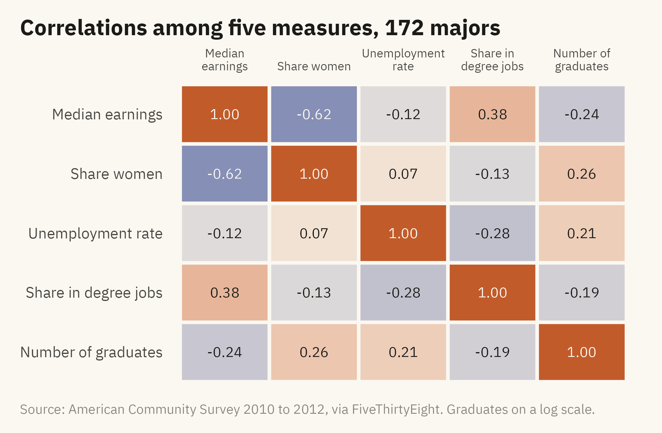
Figure 6.5 shows the correlations among five variables in the data as a grid. It shows which measures move together and nothing about cause.

vars <- m |> transmute(`Median earnings` = median, `Share women` = share_women,
                       `Unemployment rate` = unemployment_rate, `Share in degree jobs` = share_college_jobs,
                       `Number of graduates` = log10(graduates))
cm <- cor(vars, use = "pairwise.complete.obs") |> as.data.frame() |> rownames_to_column("a") |>
  pivot_longer(-a, names_to = "b", values_to = "r") |>
  mutate(a = factor(a, levels = names(vars)), b = factor(b, levels = rev(names(vars))))
ggplot(cm, aes(a, b, fill = r)) +
  geom_tile(color = mv_ink$canvas, linewidth = 1) +
  geom_text(aes(label = sprintf("%.2f", r), color = abs(r) > 0.5), size = 3, family = mv_font()) +
  scale_color_manual(values = c(`TRUE` = mv_ink$canvas, `FALSE` = mv_ink$ink), guide = "none") +
  scale_fill_gradient2(low = "#3C5A99", mid = "#F2EDE2", high = mv_accent(), limits = c(-1, 1), guide = "none") +
  scale_x_discrete(labels = label_wrap(12), position = "top") +
  labs(title = "Correlations among five measures, 172 majors", x = NULL, y = NULL, caption = mv_source(src, "Graduates on a log scale")) +
  theme_mv(grid = "none") +
  theme(axis.text.x = element_text(size = rel(0.8), lineheight = 0.9), axis.line.x = element_blank())

Figure 6.5: Correlations among five measures across 172 majors. Earnings rise with the share of graduates in jobs that need a degree and fall with the share of women. Unemployment is only weakly correlated with the other measures. A correlation grid shows which measures move together, and nothing about why. Source: American Community Survey 2010 to 2012, via FiveThirtyEight.

A correlation grid is a heatmap. Color intensity is low on the hierarchy, so the values are printed in the cells as well. The color shows the overall pattern, and the printed values give the exact figures. Both can be used when a grid has fewer than about fifty cells.

6.7 The Spread Behind the Point

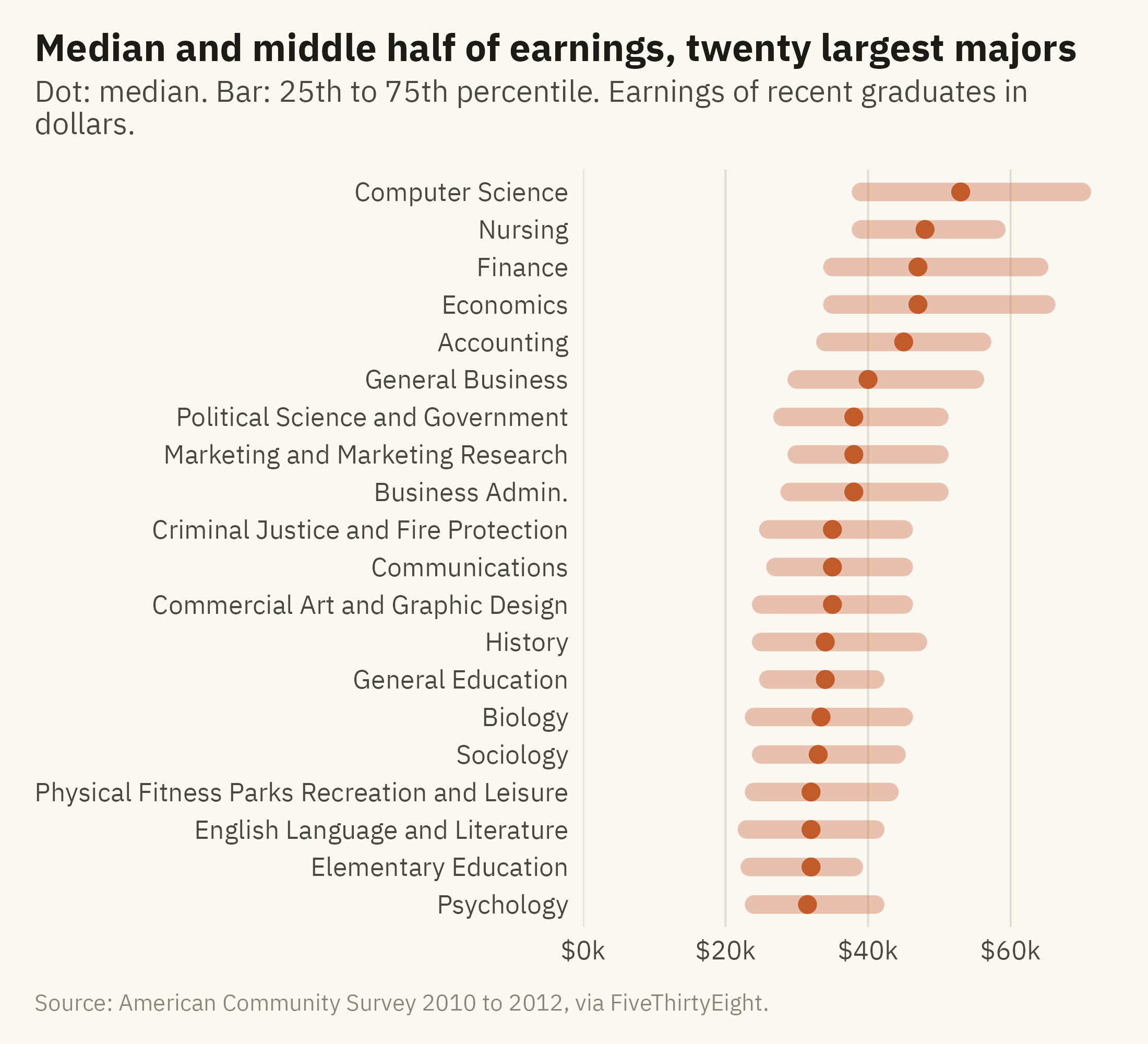
Every point in this chapter is a median. A median leaves out the range around it. Half of petroleum engineers earn less than $110,000, and a quarter earn less than $95,000. Figure 6.6 draws the middle half of earnings for the twenty largest majors. Each major is drawn as a bar from the 25th to the 75th percentile, with the median marked by a dot.

big <- m |> slice_max(graduates, n = 20) |>
  mutate(major = str_replace(major, "Business Management and Administration", "Business Admin."),
         major = fct_reorder(major, median))
ggplot(big) +
  geom_segment(aes(x = p25, xend = p75, y = major, yend = major), color = mv_accent(), linewidth = 3, alpha = 0.35, lineend = "round") +
  geom_point(aes(median, major), color = mv_accent(), size = 2.4) +
  scale_x_continuous(labels = label_dollar(scale = 1e-3, suffix = "k"), limits = c(0, NA), expand = expansion(mult = c(0, 0.04))) +
  labs(title = "Median and middle half of earnings, twenty largest majors",
       subtitle = "Dot: median. Bar: 25th to 75th percentile. Earnings of recent graduates in dollars.",
       x = NULL, y = NULL, caption = mv_source(src)) +
  theme_mv(grid = "x")

Figure 6.6: The middle half of earnings (25th to 75th percentile) for the twenty largest majors, sorted by median. The ranges overlap heavily. A nursing graduate at the 75th percentile earns more than a computer science graduate at the 25th. Source: American Community Survey 2010 to 2012, via FiveThirtyEight.

The relationship in Figure 6.1 is a relationship between majors. Each point on that plot is the median of a wide range of individual earnings. A person’s major therefore predicts that person’s earnings less well than the scatter plot suggests. Chapter 10 returns to this with methods for showing uncertainty.

6.8 The Final Version of the Chart

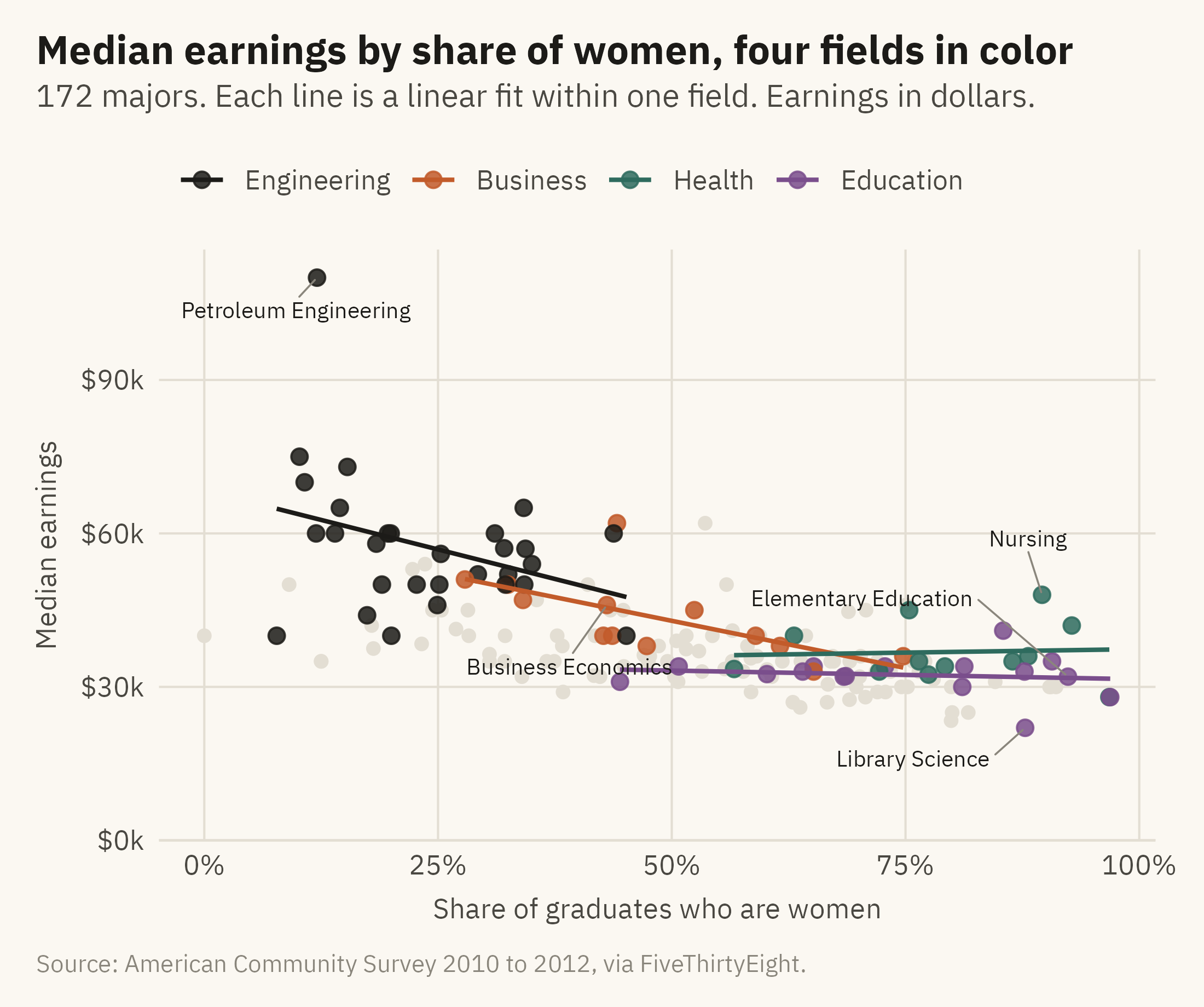
Figure 6.7 keeps all 172 points, labels the exceptions, and colors the majors in four fields. The remaining majors are in grey. A fitted line is drawn within each colored field.

four <- c("Engineering", "Business", "Health", "Education")
fin <- m |> mutate(grp = if_else(category %in% four, category, "Other"),
                   grp = factor(grp, levels = c(four, "Other")))
cols <- c(Engineering = mv_ink$ink, Business = mv_accent(), Health = "#2E6B5E", Education = "#7A4E8C", Other = mv_ink$grid)
labs_pts <- m |> filter(major %in% c("Petroleum Engineering", "Nursing", "Elementary Education", "Business Economics",
                                     "Library Science")) |>
  mutate(ny = case_when(major == "Elementary Education" ~ 18000, major == "Business Economics" ~ -12000,
                        major == "Library Science" ~ -6000, major == "Nursing" ~ 9000, TRUE ~ 0),
         nx = case_when(major == "Elementary Education" ~ -0.2, major == "Business Economics" ~ -0.04,
                        major == "Library Science" ~ -0.12, major == "Nursing" ~ -0.03, TRUE ~ 0))
ggplot(fin, aes(share_women, median, color = grp)) +
  geom_point(data = filter(fin, grp == "Other"), size = 1.6) +
  geom_point(data = filter(fin, grp != "Other"), size = 2.2, alpha = 0.85) +
  geom_smooth(data = filter(fin, grp != "Other"), method = "lm", se = FALSE, linewidth = 0.7, formula = y ~ x) +
  geom_text_repel(data = labs_pts, aes(label = major), color = mv_ink$ink, size = 2.6, family = mv_font(),
                  nudge_x = labs_pts$nx, nudge_y = labs_pts$ny,
                  min.segment.length = 0, segment.color = mv_ink$mute, segment.size = 0.3, box.padding = 0.5, seed = 3) +
  scale_color_manual(values = cols, breaks = four, name = NULL) +
  scale_x_continuous(labels = label_percent()) +
  scale_y_continuous(labels = label_dollar(scale = 1e-3, suffix = "k"), limits = c(0, NA), expand = expansion(mult = c(0, 0.05))) +
  labs(title = "Median earnings by share of women, four fields in color",
       subtitle = "172 majors. Each line is a linear fit within one field. Earnings in dollars.",
       x = "Share of graduates who are women", y = "Median earnings", caption = mv_source(src)) +
  theme_mv(grid = "y") +
  theme(panel.grid.major.x = element_line(color = mv_ink$grid, linewidth = 0.35))

Figure 6.7: Median earnings by share of women, with four fields in color and the rest in grey. Engineering is at the upper left and education at the lower right. Part of the overall slope is the distance between them. Within business the slope is steep. Within health it is flat, and nursing is the main reason. Source: American Community Survey 2010 to 2012, via FiveThirtyEight.

ImportantEthics Moment: The Sentence Under the Chart

Many readers will take a scatter plot with a downward slope as evidence of a cause. An author should expect that. “Majors with more women pay less” is a description. “Women choose low-paying majors” is a claim about choice. “Fields pay less when women enter them” is a claim about discrimination. The chart supports the first sentence and not the other two. Write the sentence the chart supports. If you believe one of the others, state it as your own claim and cite the evidence beyond the chart. Levanon, England, and Allison (2009) is an example of the kind of evidence a causal claim needs.

TipTry It Online

Two Variables at viz.marginoferrormedia.com/apps includes the majors data. Choose any two of the eight measures for the axes, a third for size, and a field to highlight. The app draws the fit and reports the correlation. A toggle shows how the correlation changes when you remove any single major. Try removing petroleum engineering.

WarningAI Reality Check: The Line Without the Cloud

Ask a model to “show the relationship between share of women and earnings.” A common first draft is a bar chart of average earnings in four or five bins of share of women. The bins leave out the spread within each bin, so the relationship appears stronger and more precise than it is. A second common draft is a scatter plot with the fitted line and no points. Both drafts present a summary in place of the data.

Ask for the points, with the line drawn over them and the outliers labeled. When the model writes a caption with the word “because,” ask it which of the three explanations in this chapter it has evidence for. In most cases it has evidence for none of them.

6.9 Putting It All Together

A relationship between two variables is read in three steps: direction, strength, and shape. A scatter plot shows all three because it draws every observation. A fitted line summarizes the direction as a slope and should be drawn with the points. Labels and size identify individual observations. Small multiples show whether the pattern holds within groups or only between them. A correlation grid shows which measures move together. None of these charts shows which variable causes the other.

6.10 Looking Ahead

Chapter 7 adds time. The questions become how a measure changed, and whether two sources that measure the same thing agree about the change. The case is crime in the United States. It is counted once from police records and once from a survey that asks people what happened to them. The two series have differed for fifty years.

6.11 Further Reading and References

Carnevale, A. P., Cheah, B., and Hanson, A. R. (2015). The Economic Value of College Majors. Georgetown University Center on Education and the Workforce. The source of the field categories and a fuller analysis of the earnings gap by major.

Casselman, B. (2014). The economic guide to picking a college major. FiveThirtyEight, September 12. The article the data was compiled for.

Cleveland, W. S., and McGill, R. (1984). The many faces of a scatterplot. Journal of the American Statistical Association, 79(388), 807–822. On what readers see in a scatter plot and how to help them.

Levanon, A., England, P., and Allison, P. (2009). Occupational feminization and pay: Assessing causal dynamics using 1950–2000 U.S. census data. Social Forces, 88(2), 865–891. The study most often cited for the claim that pay falls when women enter a field, and an example of what evidence beyond a scatter plot looks like.

Tufte, E. R. (2006). Beautiful Evidence. Graphics Press. The chapter on sparklines and the one on “corruption in evidence presentations” both bear on this chapter.

6.12 Key Terms

Scatter plot. One point per observation, positioned by two variables. Shows a relationship with every observation drawn.

Direction, strength, shape. The three features to read from a scatter plot, in that order.

Fitted line. A summary of the direction of a relationship as a slope, drawn with the points rather than in place of them.

Confidence band. The uncertainty in a fitted line, not the spread of the data.

Small multiples with a reference layer. One panel per group, with the full data in grey behind each, so panels can be compared.

Correlation grid. A heatmap of pairwise correlations with the values printed in the cells.

6.13 Exercises

Check Your Understanding

1. State the direction, strength, and shape of the relationship in Figure 6.1 in one sentence each.
2. A reader says the shaded band in Figure 6.2 shows that most majors earn within $5,000 of the line. What have they misread?
3. Why are the grey points repeated in every panel of Figure 6.4? What would be lost without them?
4. Name the three causal explanations consistent with Figure 6.1 and say which, if any, the chart supports.
5. In Figure 6.5, which pair of variables has the strongest correlation, and is it positive or negative?

Apply It

6. Using ch06-college-majors.csv, draw unemployment rate against median earnings. Describe the direction, strength, and shape, and name the three majors furthest from the trend.
7. Redraw Figure 6.1 with earnings on a log axis. Does the relationship look more or less linear? Which version would you publish, and why?
8. Compute the correlation between share of women and median earnings within each field. Rank the fields. Which has the strongest relationship, and does it have enough majors for the number to mean much?
9. Add a size variable of your choosing to Figure 6.7 and write a caption that tells the reader what the size encodes and what it adds.

Think Deeper

10. The chapter says a relationship between majors is not a relationship between people. Explain, using Figure 6.6, why a student should not treat the scatter plot as a forecast of their own earnings.
11. Suppose you wanted to test the explanation that fields pay less when women enter them. What data would you need that this chapter’s data does not have, and what chart would show the result?
12. The Ethics Moment asks for the sentence the chart supports. Write three captions for Figure 6.7, one that states only what the chart supports, one that overclaims in the direction of choice, and one that overclaims in the direction of discrimination, and mark the words that make the difference.